Euler’s Method

Euler’s Method#

Most differential equations cannot be solved explicitly with elementary functions. So what do we do? Numerical methods are algorithms to numerically approximate solutions of differential equations and Euler’s method is the most basic numerical method. The idea is simple: use the equation \(y' = f(t,y)\) to construct the tangent line to the unknown solution \(y(t)\) at a given point \(t\), approximate the solution nearby \(y(t+h)\) and repeat.

Formulation#

Consider a first order differential equation \(y' = f(t,y)\) with initial value \(y(t_0) = y_0\). Use the tangent line of the solution to approximate values near \(t = t_0\)

\[ y(t) \approx y_0 + f(t_0,y_0)(t - t_0) \]

In particular, choose a step size \(h = t_1 - t_0\) and define

\[ y_1 = y_0 + f(t_0,y_0)(t_1 - t_0) \]

Repeating the process defines a recursive sequence

\[ y_{n+1} = y_n + f(t_n,y_n)(t_{n+1} - t_n) \ , \ \ y(t_0) = y_0 \]

such that \(y_n \approx y(t_n)\) is an approximation of the solution \(y(t)\) at \(t=t_n\). Note that we usually choose the same step size \(h = t_{n+1} - t_n\) for all \(n\) so that \(t_n = t_0 + nh\).

Implementation#

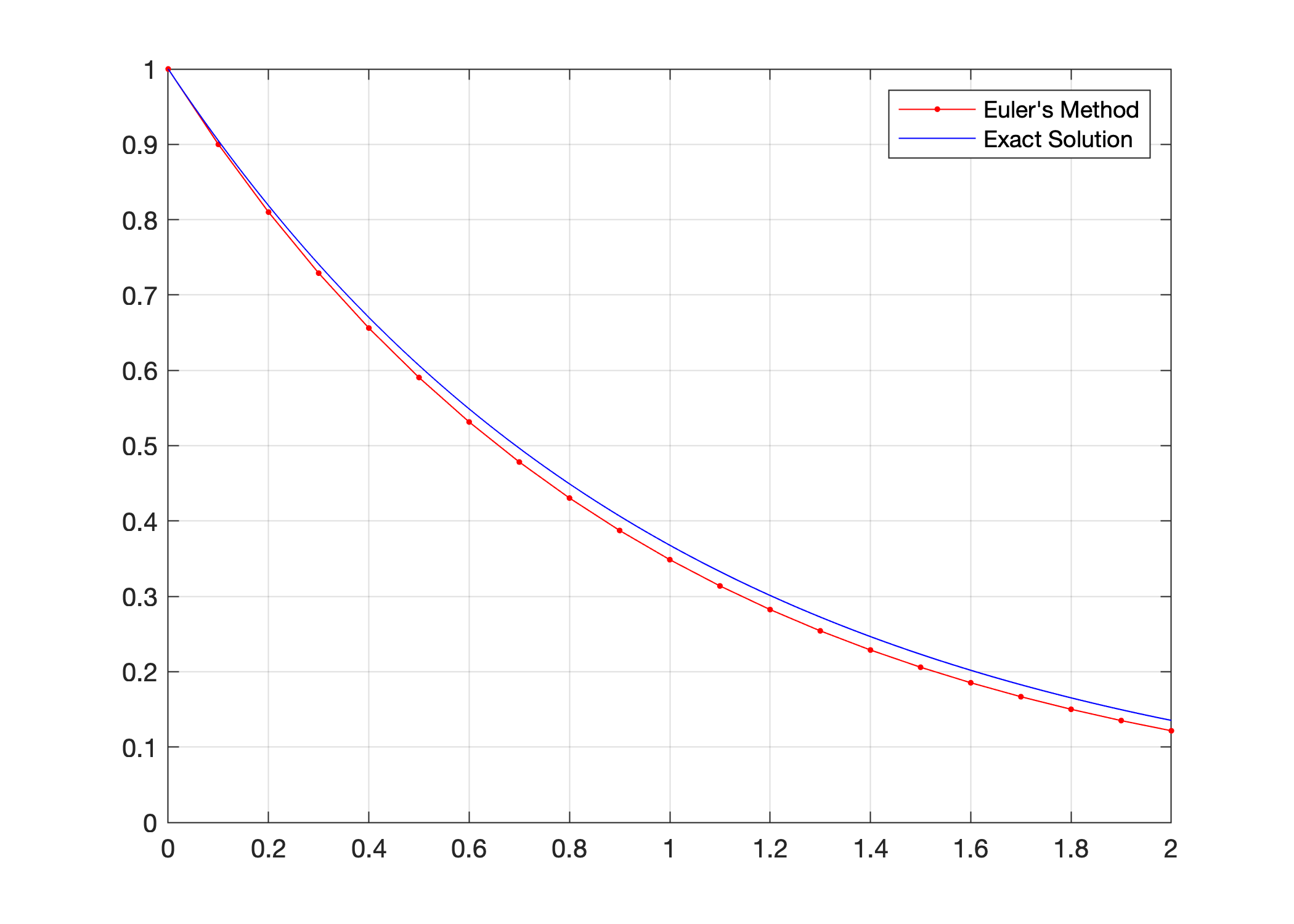
Consider the familiar equation \(y' = -y\), \(y(0) = 1\). We know the exact solution is \(y(t) = e^{-t}\). Let’s compute the approximation by Euler’s method and compare to the exact answer.

f = @(t,y) -y;
t0 = 0; tf = 2; h = 0.1;
t = t0:h:tf;
y0 = 1;

y = zeros(size(t));
y(1) = y0;

for n = 1:(length(t)-1)
    y(n+1) = y(n) + f(t(n),y(n))*h;
end

t_exact = linspace(t0,tf,200);
y_exact = exp(-t_exact);

plot(t,y,'r.-',t_exact,y_exact,'b')
legend("Euler's Method","Exact Solution")
ylim([0,1]), grid on

Let’s take a closer look at each step in the script above:

Step 1: Setup the differential equation, initial value and step size

f = @(t,y) -y;
t0 = 0; tf = 2; h = 0.1;
t = t0:h:tf;
y0 = 1;

Define the right hand side of the differential equation \(y' = f(t,y)\) as a function f
Enter the intial \(t\) value t0
Choose an interval \([t_0,t_f]\) over which to compute the approximation by setting a value for tf
Choose the step size h
Create the vector of values from \(t_0\) to \(t_f\) incremented by \(h\) (ie. \(t_n = t_0 + nh\))
Enter the initial value y0 (corresponding to \(y(t_0) = y_0\))

Step 2: Initialize the vector of \(y\) values

y = zeros(size(t));
y(1) = y0;

Initialize a vector y of zeros of same size as the vector t
Enter the initial value \(y_0\) for the first entry of vector y

Step 3: Implement Euler’s method

for n = 1:(length(t)-1)
    y(n+1) = y(n) + f(t(n),y(n))*h;
end

Compute \(y_{n+1} = y_n + f(t_n,y_n)(t_{n+1} - t_n)\) for each \(n\)
The value y(n) corresponds to \(y_{n-1}\) in the sequence \(y_0,y_1,y_2,\dots\) since y starts at index 1
The for loop updates the entry y(n+1) in the vector y each time through the loop

Step 4: Compute the exact solution

t_exact = linspace(t0,tf,200);
y_exact = exp(-t_exact);

Create a vector of \(t\) values from \(t_0\) to \(t_f\) to construct the exact solution
Compute the \(y\) values using the formula for the exact solution \(y(t) = e^{-t}\)

Step 5: Plot the result

plot(t,y,'r.-',t_exact,y_exact,'b')
legend("Euler's Method","Exact Solution")
ylim([0,1]), grid on

Plot the approximations generated by Euler’s method as red dots connected by a solid line 'r.-'
Plot the exact solution as a blue line 'b'
Add a legend, restrict the range of the \(y\) axis to the interval \([0,1]\) and add a grid

`odeEuler`#

We will repeat the exact same code in steps 2 and 3 above every time we implement Euler’s method and so we should package those lines of code into a function so that we can easily reuse the code. Let’s create a function called odeEuler which takes input parameters:

f is a function which represents the right hand side of a differential equation \(y' = f(t,y)\)
t is a vector of \(t\) values from \(t_0\) to \(t_f\)
y0 is the initial value \(y(t_0) = y_0\)

The function returns vectors T and Y where:

T is the same as the input vector t
Y is the vector of \(y\) values computed by Euler’s method

function [T,Y] = odeEuler(f,t,y0)

T = t;
Y = zeros(size(T));
Y(1) = y0;
for n = 1:(length(t)-1)
    Y(n+1) = Y(n) + f(T(n),Y(n))*(T(n+1) - T(n));
end

end

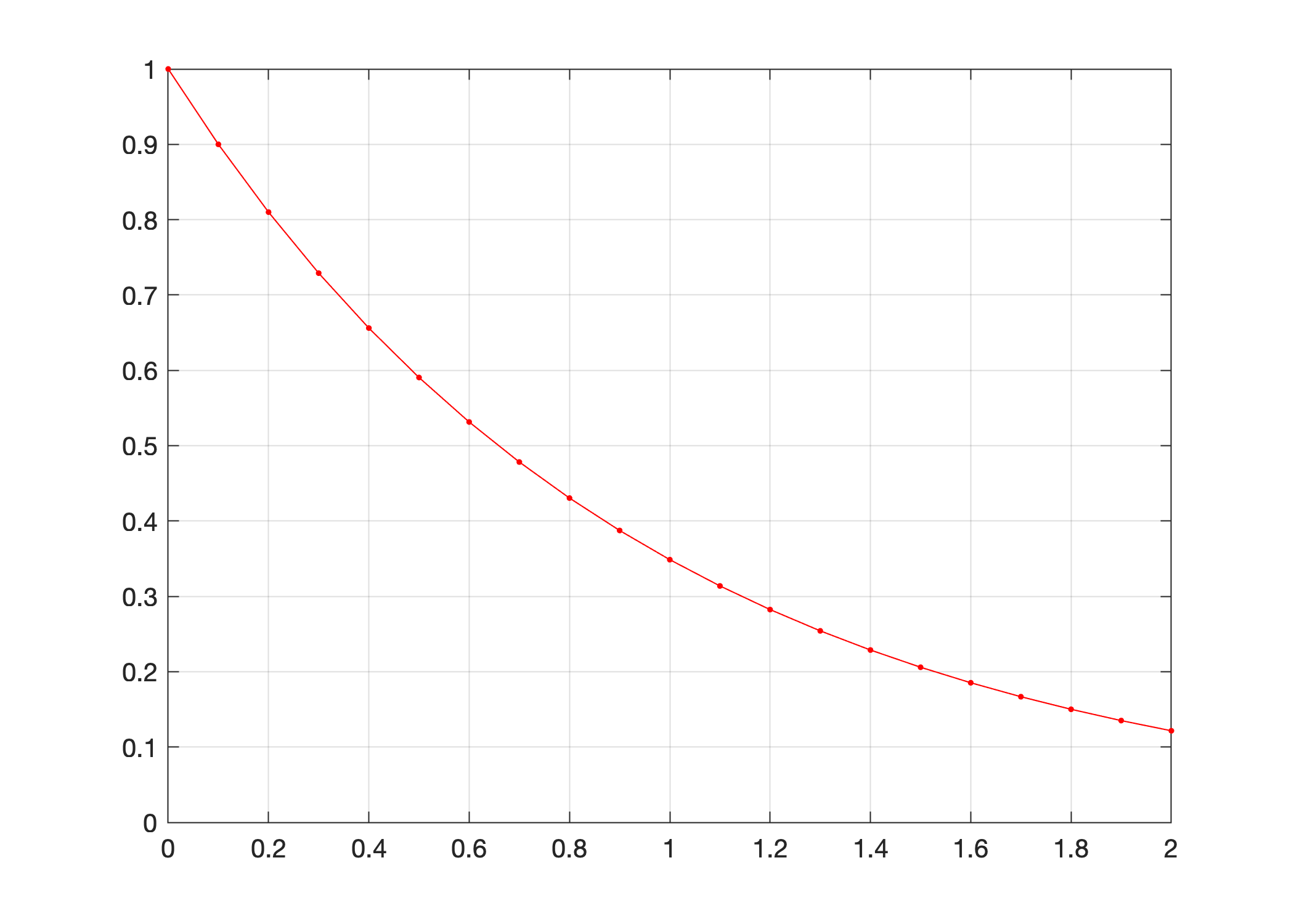
Let’s use odeEuler to plot the approximation of \(y' = y\), \(y(0)=1\).

f = @(t,y) -y;
t0 = 0; tf = 2; h = 0.1; t = t0:h:tf; y0 = 1;
[T,Y] = odeEuler(f,t,y0);
plot(T,Y,'r.-'), ylim([0,1]), grid on

Note

Copy and paste the code for the function odeEuler into a new script and save the file in your MATLAB development environment as odeEuler.m. The file odeEuler.m must be saved to the current folder to use it in other scripts in the same folder. Also the function odeEuler is designed to accept and return the same input and output parameters as the MATLAB function ode45. We’ll see ode45 in later sections.

Examples#

Example: Euler’s method and slope fields

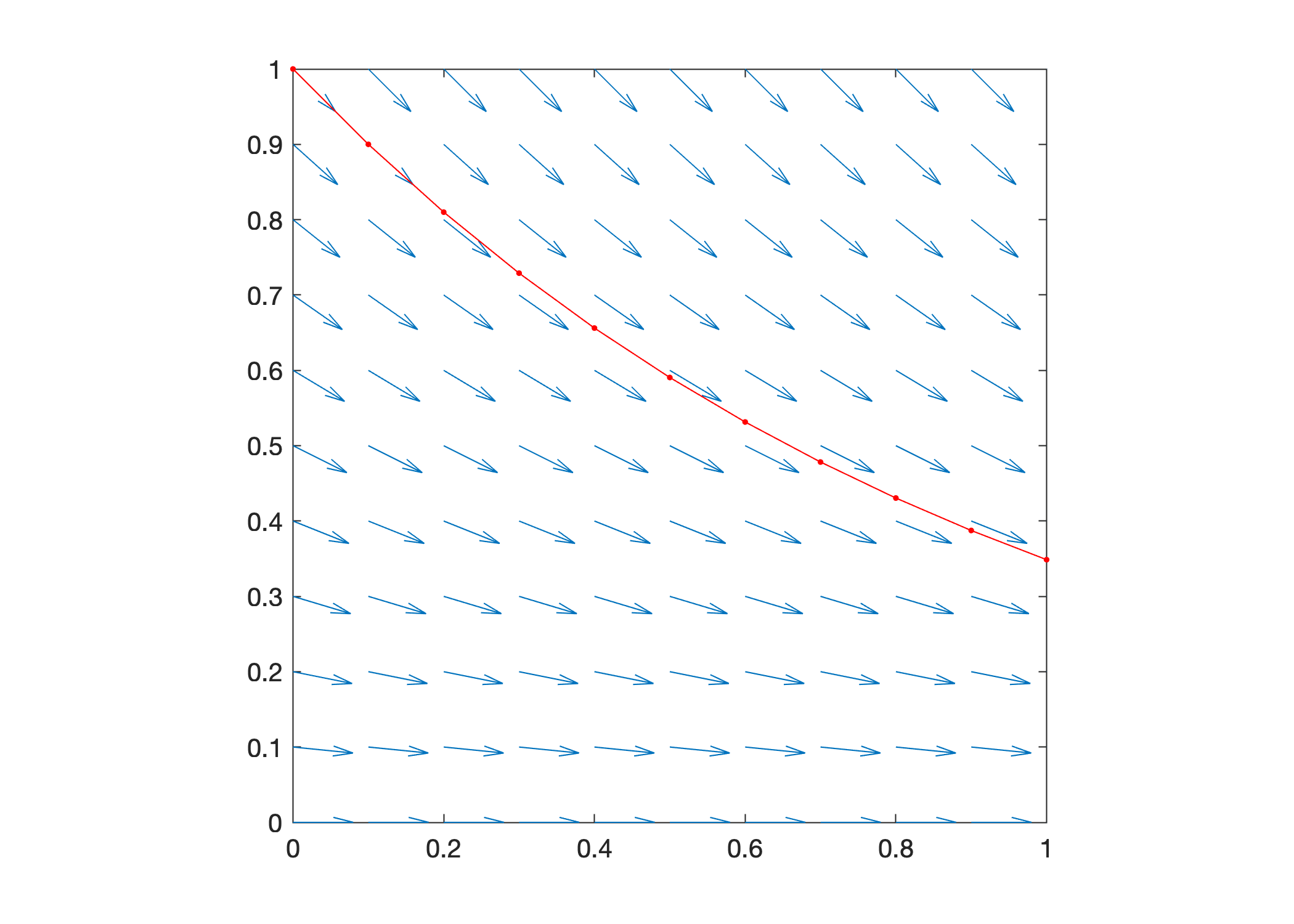
Euler’s method is an iterative method which generates approximations of solutions of differential equations by simply following the slopes in a slope field. Plot an approximation of \(y' = y\), \(y(0) = 1\) along with the slope field to view the realtionship between them.

f = @(t,y) -y;
t0 = 0; tf = 2; h = 0.1; t = t0:h:tf; y0 = 1;
y = 0:h:1;
slopefield(f,t,y), hold on
[T,Y] = odeEuler(f,t,y0);
plot(T,Y,'r.-'), hold off

Example: Nonlinear, nonseparable equations

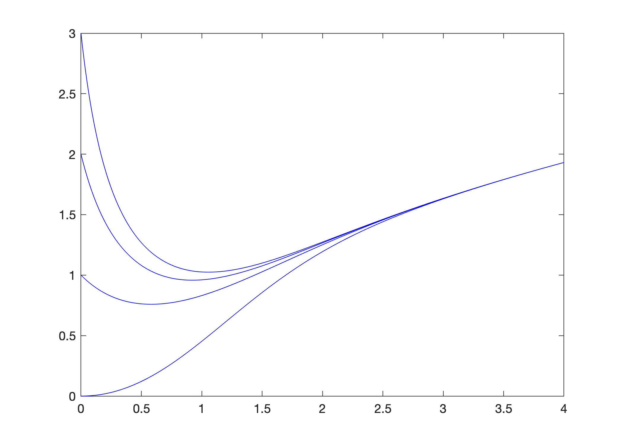
As we have noted multiple times before, most differential equations are impossible to solve explicitly with elementary functions. We have methods to analytically solve linear equations and separable equations and so let’s use Euler’s method to approximate solutions for an equation that is neither linear nor separable. Plot an approximation of \(y' = t - y^2\) for each initial value \(y(0)=0,1,2,3\).

f = @(t,y) t - y.^2;
t0 = 0; tf = 4; h = 0.01; t = t0:h:tf;
[T,Y0] = odeEuler(f,t,0); plot(T,Y0,'b'), hold on
[T,Y1] = odeEuler(f,t,1); plot(T,Y1,'b')
[T,Y2] = odeEuler(f,t,2); plot(T,Y2,'b')
[T,Y3] = odeEuler(f,t,3); plot(T,Y3,'b'), hold off

Example: Use a for loop to plot many solutions

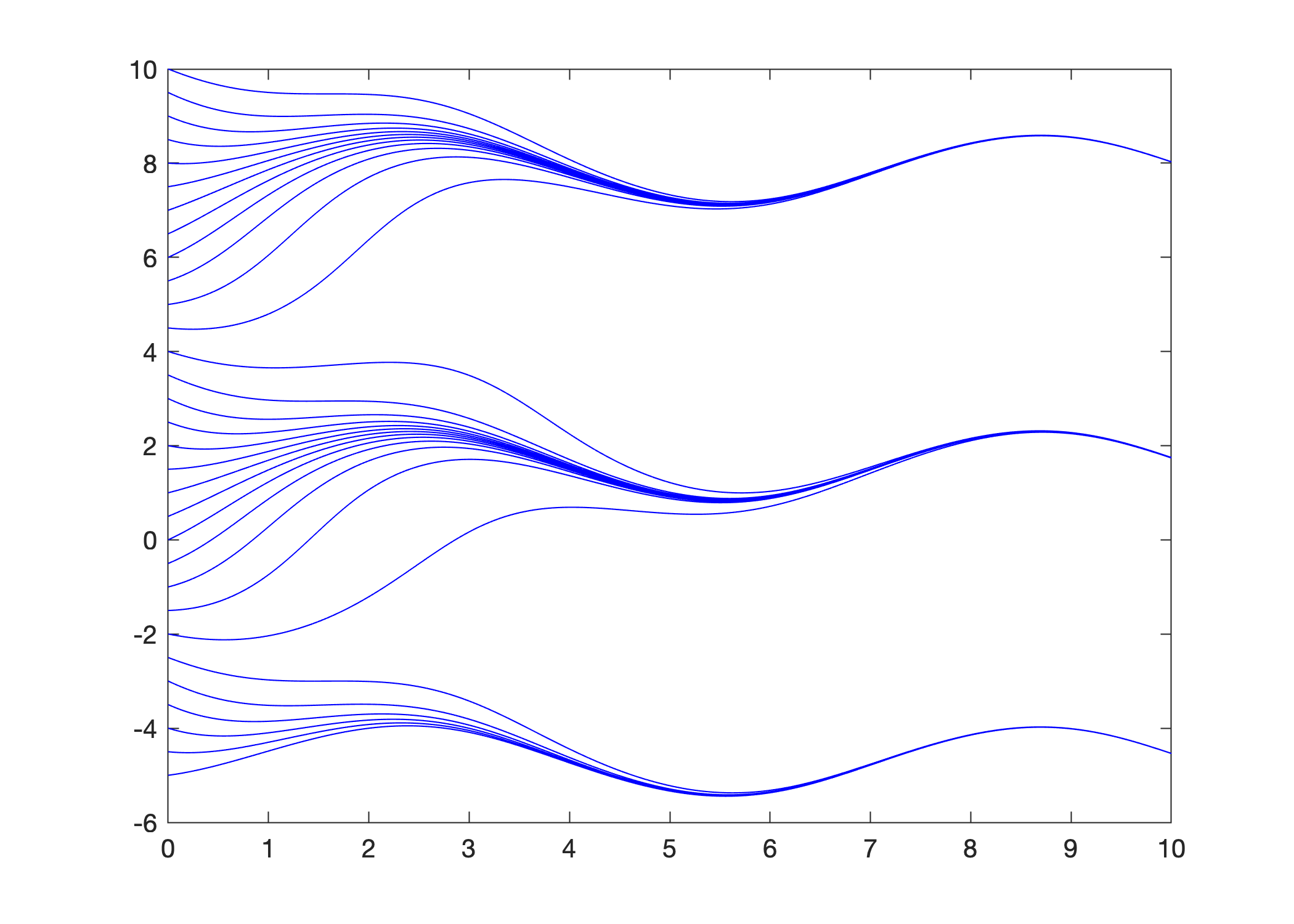
In the previous example, we repeated the same commands to approximate and plot solutions for differential initial values. Let’s now use a for loop to plot an approximations of \(y' = \sin(t) + \cos(y)\) for each initial value \(y(0) = y_0\) from \(y_0 = -5\) to \(y_0 = 10\) incremented by \(0.5\).

f = @(t,y) sin(t) + cos(y);
t0 = 0; tf = 10; h = 0.01; t = t0:h:tf;
for y0=-5:0.5:10
    [T,Y] = odeEuler(f,t,y0);
    plot(T,Y,'b'), hold on
end
hold off

Error Analysis#

Under construction