Fourier Series

import numpy as np
import matplotlib.pyplot as plt
import scipy.integrate as spi

Definition

Let \(f(x)\) be a (piecewise) continuous function on the interval \([-L,L]\). The Fourier series of \(f(x)\) is

\[ f(x) = \frac{a_0}{2} + \sum_{n=1}^{\infty} a_n \cos \left( \frac{n \pi x}{L} \right) + \sum_{n=1}^{\infty} b_n \sin \left( \frac{n \pi x}{L} \right) \]

where the coefficients are given by the integrals

\[ a_0 = \frac{1}{L} \int_{-L}^L f(x) dx \]

\[ a_n = \frac{1}{L} \int_{-L}^L f(x) \cos \left( \frac{n \pi x}{L} \right) dx \]

\[ b_n = \frac{1}{L} \int_{-L}^L f(x) \sin \left( \frac{n \pi x}{L} \right) dx \]

Computing Coefficients

Use the SciPy funciton scipy.integrate.quad (see documentation) to numerically approximate a definite integral. For example, let’s approximate the integral

\[ \int_0^{1} \sin(x^2) dx \]

f = lambda x: np.sin(x**2)
a = 0
b = 1
I,error = spi.quad(f,a,b)

The function returns the approximation and an upper bound for the error:

I

0.3102683017233811

error

3.444670123846428e-15

Let’s use the function scipy.integrate.quad to approximate first few Fourier coefficients of the function \(f(x) = 1 - x^2\) on the interval \([-1,1]\).

f = lambda x: 1 - x**2
L = 1

I0,_ = spi.quad(f,-L,L)
a0 = 1/L*I0
a0

1.3333333333333335

integrand_a1 = lambda x: f(x)*np.cos(np.pi*x/L)
Ia1,_ = spi.quad(integrand_a1,-L,L)
a1 = 1/L*Ia1
a1

0.40528473456935127

integrand_a2 = lambda x: f(x)*np.cos(2*np.pi*x/L)
Ia2,_ = spi.quad(integrand_a2,-L,L)
a2 = 1/L*Ia2
a2

-0.10132118364233778

integrand_b1 = lambda x: f(x)*np.sin(np.pi*x/L)
Ib1,_ = spi.quad(integrand_b1,-L,L)
b1 = 1/L*Ib1
b1

0.0

integrand_b2 = lambda x: f(x)*np.sin(2*np.pi*x/L)
Ib2,_ = spi.quad(integrand_b2,-L,L)
b2 = 1/L*Ib2
b2

0.0

Of course, all the coefficients \(b_n = 0\) since \(f(x)\) is an even function.

The function fourier takes input parameters f, L and N, and returns a tuple (a0,a,b) where:

• f is a Python function representing \(f(x)\)

• L defines the interval \([-L,L]\)

• N is the number of coefficients to compute

• a0 is the constant term \(a_0\) in the Fourier series

• a is a NumPy array of length \(N\) of Fourier coefficients \(a_1,\dots,a_N\)

• b is a NumPy array of length \(N\) of Fourier coefficients \(b_1,\dots,b_N\)

def fourier(f,L,N):
    a = np.zeros(N)
    b = np.zeros(N)
    I,_ = spi.quad(f,-L,L)
    a0 = 1/L*I
    for n in range(1,N+1):
        integrand = lambda x: f(x)*np.cos(n*np.pi*x/L)
        I,_ = spi.quad(integrand,-L,L)
        a[n-1] = 1/L*I
        integrand = lambda x: f(x)*np.sin(n*np.pi*x/L)
        I,_ = spi.quad(integrand,-L,L)
        b[n-1] = 1/L*I
    return a0,a,b

For example, let’s apply fourier to \(f(x) = 1 - x^2\) on \([-1,1]\) and recover the coefficients computed in the example in the previous section above.

f = lambda x: 1 - x**2
L = 1
N = 5
a0,a,b = fourier(f,L,N)

a0

1.3333333333333335

a

array([ 0.40528473, -0.10132118,  0.04503164, -0.0253303 ,  0.01621139])

b

array([0., 0., 0., 0., 0.])

Now let’s try an example where \(f(x)\) is a sum of sine and cosine functions to verify that the function fourier simply recovers the coefficients in the definition of \(f(x)\).

f = lambda x: 1 + 3*np.sin(np.pi*x) + np.cos(np.pi*x) + 3*np.sin(3*np.pi*x)
L = 1
N = 4
a0,a,b = fourier(f,L,N)

a0

2.0000000000000004

a

array([ 1.00000000e+00, -8.32667268e-17, -2.77555756e-17, -5.55111512e-17])

b

array([ 3.00000000e+00,  0.00000000e+00,  3.00000000e+00, -3.33066907e-16])

When programming in Python, we can interpret numbers such as \(10^{-16}\) as 0 therefore we have \(a_0 = 2\), \(a_1 = 1\), \(a_2 = a_3 = a_4 = 0\), \(b_1 = 3\), \(b_2 = b_4 = 0\) and \(b_3 = 3\).

Computing Series

The function fouriersum takes the output a0, a and b from the function fourier along with array x and number L and returns the array of \(y\) values given by the sum

\[ \frac{a_0}{2} + \sum_{n=1}^N a_n \cos \left( \frac{n \pi x}{L} \right) + \sum_{n=1}^N b_n \sin \left( \frac{n \pi x}{L} \right) \]

def fouriersum(a0,a,b,x,L):
    cosine_sum = sum([a[n-1]*np.cos(n*np.pi*x/L) for n in range(1,len(a)+1)])
    sine_sum = sum([b[n-1]*np.sin(n*np.pi*x/L) for n in range(1,len(b)+1)])
    return a0/2 + cosine_sum + sine_sum

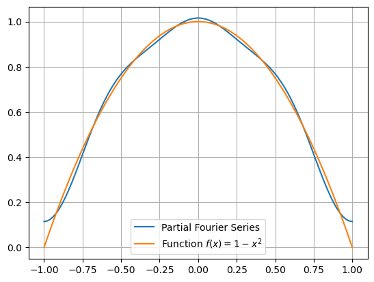
Let’s plot the function \(f(x) = 1 - x^2\) along with the partial Fourier series up to \(N=3\).

f = lambda x: 1 - x**2
L = 1
N = 3
a0,a,b = fourier(f,L,N)
x = np.linspace(-L,L,100)
y = fouriersum(a0,a,b,x,L)
plt.plot(x,y,label="Partial Fourier Series")
plt.plot(x,f(x),label="Function $f(x) = 1-x^2$")
plt.grid(True), plt.legend()
plt.show()

Examples

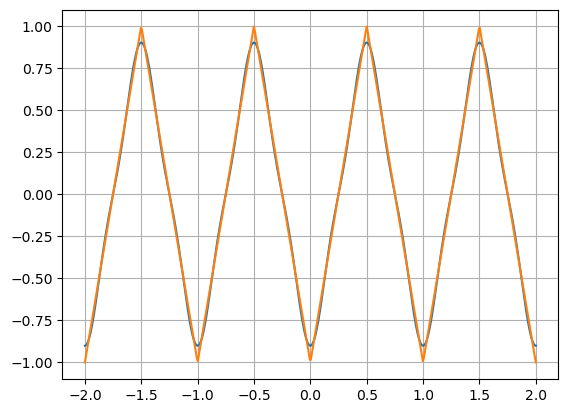
Sawtooth Wave

import scipy.signal as sps

f = lambda x: sps.sawtooth(2*np.pi*x,width=0.5)
L = 2
a0,a,b = fourier(f,L,15)
x = np.linspace(-L,L,500)
y = fouriersum(a0,a,b,x,L)
plt.plot(x,y)
plt.plot(x,f(x))
plt.grid(True)
plt.show()

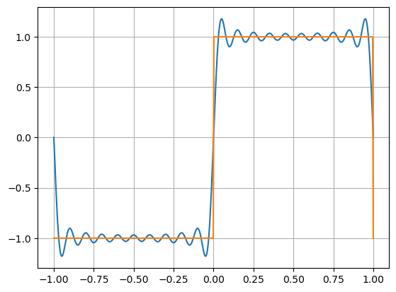
Square Wave

f = lambda x: sps.square(np.pi*x)
L = 1
N = 20
a0,a,b = fourier(f,L,N)
x = np.linspace(-L,L,500)
y = fouriersum(a0,a,b,x,L)
plt.plot(x,y)
plt.plot(x,f(x))
plt.grid(True)
plt.show()