Laplace Equation

import numpy as np
import matplotlib.pyplot as plt

The Laplace equation is given by

\[ \frac{\partial^2 u}{\partial x^2} + \frac{\partial^2 u}{\partial y^2} = 0 \ , \ \ 0 \leq x \leq L_x \ , \ \ 0 \leq y \leq L_y \]

where the solution \(u(x,y)\) is defined on the rectangular domain \([0,L_x] \times [0,L_y]\).

Boundary Conditions

Both variables \(x\) and \(y\) are spatial and there is no time variable \(t\). Therefore there are only boundary conditions in the \(x\) and \(y\) directions and no initial condition to consider.

Dirichlet boundary conditions specify the values of the solution at the endpoints:

\[ u(0,y) = f_0(y) \hspace{20mm} u(L_x,y) = f_1(y) \]

\[ u(x,0) = g_0(x) \hspace{20mm} u(x,L_y) = g_1(x) \]

Neumann boundary conditions specify the values of the derivative of the solution at the endpoints:

\[ u_x(0,y) = p_0(y) \hspace{20mm} u_x(L_x,y) = p_1(y) \]

\[ u_y(x,0) = q_0(x) \hspace{20mm} u_y(x,L_y) = q_1(x) \]

When boundary conditions include both Dirichlet and Neumann conditions we call them mixed boundary conditions.

Discretization

Choose the number of steps \(N_x\) in the \(x\) direction and \(N_y\) steps in the \(y\) direction. These choices determine the step sizes \(\Delta x\) and \(\Delta y\), and create a grid of points:

\[\begin{split} \begin{align} x_n &= n \Delta x \ , \ \ n = 0,1, \dots, N_x \ , \ \ \Delta x = \frac{L_x}{N_x} \\ y_m &= m \Delta y \ , \ \ m = 0,1, \dots, N_y \ , \ \ \Delta y = \frac{L_y}{N_y} \end{align} \end{split}\]

The domain of the solution \(u(x,y)\) is the rectangle \([0,L_x] \times [0,L_y]\). The goal of a finite difference method is to compute the matrix

\[ U = [u_{n,m}] \]

which gives approximations of the solution \(u(x,y)\) on the grid of points:

\[ u_{n,m} \approx u(x_n,y_m) = u(n \Delta x,m \Delta y) \]

Finite Difference Formula

Apply the central difference formula to both \(u_{xx}\) and \(u_{yy}\) at position \(x_n\) and \(y_m\)

\[ \frac{u(x_{n+1},y_m) - 2 u(x_n,y_m) + u(x_{n-1},y_m)}{(\Delta x)^2} + O((\Delta x)^2) \hspace{40mm} \]

\[ + \frac{u(x_n,y_{m+1}) - 2 u(x_n,y_m) + u(x_n,y_{m-1})}{(\Delta y)^2} + O((\Delta y)^2) = 0 \]

Rearrange to get the finite difference equation

\[ u_{n,m} = \frac{ (\Delta y)^2 \left( u_{n+1,m} + u_{n-1,m} \right) + (\Delta x)^2 \left( u_{n,m+1} + u_{n,m-1} \right) }{2 \left((\Delta x)^2 + (\Delta y)^2 \right)} \]

Note that if \(\Delta x = \Delta y\) then the formula simplifies to

\[ u_{n,m} = \frac{u_{n+1,m} + u_{n-1,m} + u_{n,m+1} + u_{n,m-1}}{4} \]

and the value at position \((x_n,y_m)\) is the average of the values in adjacent positions.

Dirichlet Boundary Conditions

Formulation

Consider the Laplace equation with Dirichlet boundary conditions:

\[ u(0,y) = f_0(y) \hspace{20mm} u(L_x,y) = f_1(y) \]

\[ u(x,0) = g_0(x) \hspace{20mm} u(x,L_y) = g_1(x) \]

It is possible to setup a large system of linear equations to numerically solve the Laplace equation however another method is to approximate the solution iteratively. In particular, define a sequence of matrices \(U_0,U_1,U_2,\dots\) where \(U_0 = [u_{n,m}^0]\) is the matrix of size \((N_x + 1) \times (N_y + 1)\) with boundary values given by the boundary conditions

\[ u^0_{0,m} = f_0(y_m) \ \ , \ \ u^0_{N_x,m} = f_1(y_m) \ \ , \ \ u^0_{n,0} = g_0(x_n) \ \ , \ \ u^0_{n,N_y} = g_1(x_n) \]

and all other values in the interior of the matrix are 0s:

\[ u_{n,m}^0 = 0 \ \ , \ \ 0 < n < N_x \ \ , \ \ 0 < m < N_y \]

Given the \(k\)th matrix \(U_k = [u_{n,m}^k]\), compute the next matrix \(U_{k+1} = [u_{n,m}^{k+1}]\) by again setting the boundary values

\[ u^{k+1}_{0,m} = f_0(y_m) \ \ , \ \ u^{k+1}_{N_x,m} = f_1(y_m) \ \ , \ \ u^{k+1}_{n,0} = g_0(x_n) \ \ , \ \ u^{k+1}_{n,N_y} = g_1(x_n) \]

and then computing the finite difference formula

\[ u^{k+1}_{n,m} = \frac{ (\Delta y)^2 \left( u^k_{n+1,m} + u^k_{n-1,m} \right) + (\Delta x)^2 \left( u^k_{n,m+1} + u^k_{n,m-1} \right) }{2 \left((\Delta x)^2 + (\Delta y)^2 \right)} \ \ , \ \ 0 < n < N_x \ \ , \ \ 0 < m < N_y \]

Iterate until the average squared difference \(\Delta U_k\) from iteration \(k\) to \(k+1\) is less than some set value \(D\):

\[ \Delta U_k = \sqrt{\frac{1}{(N_x+1)(N_y+1)} \sum_{n=0}^{N_x} \sum_{m=0}^{N_y} \left( u^{k+1}_{n,m} - u^k_{n,m} \right)^2 } < D \]

Implementation

The function laplaceD takes input parameters f0, f1, g0, g1, Lx, Ly, Nx, Ny, D and max_iter where:

• f0 is a Python function which represents the Dirichlet boundary condition \(u(0,y) = f_0(y)\)

• f1 is a Python function which represents the Dirichlet boundary condition \(u(L_x,y) = f_1(y)\)

• g0 is a Python function which represents the Dirichlet boundary condition \(u(x,0) = g_0(x)\)

• g1 is a Python function which represents the Dirichlet boundary condition \(u(x,L_y) = g_1(x)\)

• Lx and Ly define the domain \([0,L_x] \times [0,L_y]\)

• Nx and Ny are the number of steps in \(x\) and \(y\) directions of the discretization respectively

• D is the stopping criteria \(\Delta U_k < D\)

• max_iter is the maximum number of iterations before the iteration is forced to stop

The function returns the matrix \(U = [u_{n,m}]\) of size \((N_x + 1) \times (N_y + 1)\) of approximations \(u_{n,m} \approx u(x_n,y_m)\).

Set default values Lx=1, Ly=1, Nx=50, Ny=50, D=0.00001 and max_iter=5000.

def laplaceD(f0,f1,g0,g1,Lx=1,Ly=1,Nx=50,Ny=50,D=0.00001,max_iter=5000):
    U = np.zeros([Nx + 1,Ny + 1])
    dx = Lx/Nx
    dy = Ly/Ny
    for n in range(Nx + 1):
        U[n, 0] = g0(n*dx)
        U[n,Ny] = g1(n*dx)
    for m in range(Ny + 1):
        U[0, m] = f0(m*dy)
        U[Nx,m] = f1(m*dy)
    for k in range(max_iter):
        Uk = U.copy()
        for n in range(1,Nx):
            for m in range(1,Ny):
                U[n,m] = (dy**2*(Uk[n+1,m] + Uk[n-1,m]) + dx**2*(Uk[n,m+1] + Uk[n,m-1]))/(2*dx**2 + 2*dy**2)
        dU = np.sqrt(np.sum((Uk - U)**2)/(Nx + 1)/(Ny + 1))
        if dU < D:
            break
    if k == max_iter - 1:
        print("Exceeded maximum iterations.")
    else:
        print(f"Found approximation U with dUk = {dU} after k = {k} iterations.")
    return U

Note that the row index of \(U\) corresponds to the variable \(x\). Therefore if we want to visualize the solution with \(x\) in the horizontal direction and \(y\) increasing in the vertical direction then we need to plot the transpose \(U^T\) with the \(y\) axis flipped. Let’s write a function which does this.

def plot_laplace(U):
    W = np.flip(U.T,axis=0)
    plt.imshow(W,cmap='RdBu_r')
    M = np.max(np.abs(U))
    plt.clim([-M,M]), plt.axis('off'), plt.colorbar()
    plt.show()

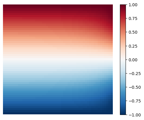
Approximate the solution for \(u(x,0) = u(0,y) = u(1,y) = 0\) and \(u(x,1) = 1\). Note that boundary conditions are always defined as Python functions.

f0 = lambda y: 0.
f1 = lambda y: 0.
g0 = lambda x: 0.
g1 = lambda x: 1.
U = laplaceD(f0,f1,g0,g1)
plot_laplace(U)

Found approximation U with dUk = 9.981637201200734e-06 after k = 1858 iterations.

Examples

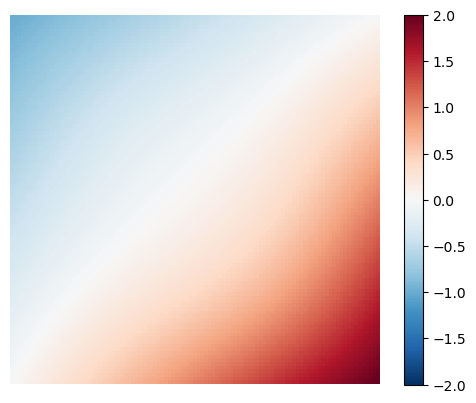
Example 1. Compute the solution for \(u(x,0) = 2x\), \(u(x,1) = x - 1\), \(u(0,y) = -y\), \(u(1,y) = 2(1 - y)\). Use \(N_x=N_y=100\) and \(D=0.0001\).

f0 = lambda y: -y
f1 = lambda y: 2*(1 - y)
g0 = lambda x: 2*x
g1 = lambda x: x - 1
U = laplaceD(f0,f1,g0,g1,Nx=100,Ny=100,D=0.0001)
plot_laplace(U)

Found approximation U with dUk = 9.995969768115448e-05 after k = 1456 iterations.

Example 2. Compute the solution for \(u(x,0) = x^2 - 1\), \(u(x,1) = x^2\), \(u(0,y) = y^2 - 1\), \(u(1,y) = y^2\). Use \(D = 0.0001\).

f0 = lambda y: y**2 - 1
f1 = lambda y: y**2
g0 = lambda x: x**2 - 1
g1 = lambda x: x**2
U = laplaceD(f0,f1,g0,g1,D=0.0001)
plot_laplace(U)

Found approximation U with dUk = 9.984942556051082e-05 after k = 665 iterations.

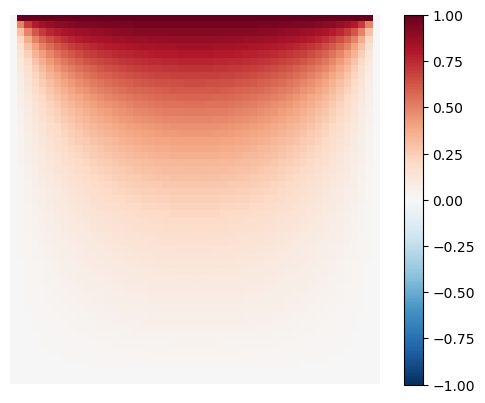
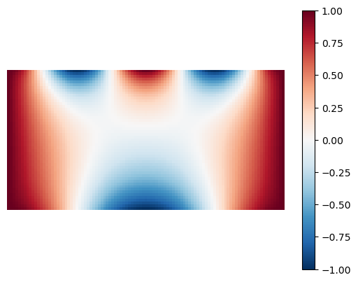
Example 3. Compute the solution for boundary conditions \(u(x,0) = \cos(\pi x)\), \(u(x,1) = \cos(2 \pi x)\), \(u(0,y) = 1\) and \(u(2,y) = 1\). Use \(N_x=100\).

f0 = lambda y: 1.
f1 = lambda y: 1.
g0 = lambda x: np.cos(np.pi*x)
g1 = lambda x: np.cos(2*np.pi*x)
U = laplaceD(f0,f1,g0,g1,Lx=2,Nx=100)
plot_laplace(U)

Found approximation U with dUk = 9.99448579108248e-06 after k = 1407 iterations.

Neumann Boundary Conditions

Formulation

Consider the Laplace equation with Neumann boundary condition \(u_x(0,y) = p_0(y)\). Apply the central difference formula:

\[ u_x(0,y) = \frac{u(\Delta x,y) - u(-\Delta x,y)}{2 \Delta x} + O((\Delta x)^2) \]

Introduce the “ghost” value \(u_{-1,m}\) and write the formula

\[ p_0(y_m) = \frac{u_{1,m} - u_{-1,m}}{2 \Delta x} \]

and rearrange

\[ u_{-1,m} = u_{1,m} - 2 \Delta x p_0(y_m) \]

The finite difference formula at \(x=0\) and \(y=y_m\) is given by

\[ u_{0,m} = \frac{ (\Delta y)^2 \left( u_{1,m} + u_{-1,m} \right) + (\Delta x)^2 \left( u_{0,m+1} + u_{0,m-1} \right) }{2 \left((\Delta x)^2 + (\Delta y)^2 \right)} \]

and rearrange to get

\[ u_{0,m} = \frac{ 2 (\Delta y)^2 \left(u_{1,m} - \Delta x p_0(y_m) \right) + (\Delta x)^2 \left( u_{0,m+1} + u_{0,m-1} \right) }{2 \left((\Delta x)^2 + (\Delta y)^2 \right)} \]

Consider the Laplace equation with Neumann boundary condition \(u_x(L_x,y) = p_1(y)\). The central difference formula gives an expression for the “ghost” value \(u_{N_x + 1,m}\):

\[ u_{N_x + 1,m} = u_{N_x - 1,m} + 2 \Delta x p_1(y_m) \]

and the finite difference formula at \(x=L_x\) and \(y=y_m\) is given by

\[ u_{N_x,m} = \frac{ 2 (\Delta y)^2 \left( u_{N_x - 1,m} + \Delta x p_1(y_m) \right) + (\Delta x)^2 \left( u_{N_x,m+1} + u_{N_x,m-1} \right) }{2 \left((\Delta x)^2 + (\Delta y)^2 \right)} \]

Consider the Laplace equation with Neumann boundary condition \(u_y(x,0) = q_0(x)\). The central difference formula gives an expression for the “ghost” value \(u_{n,-1}\):

\[ u_{n,-1} = u_{n,1} - 2 \Delta y q_0(x_n) \]

and the central difference formula at \(x=x_n\) and \(y=0\) is given by

\[ u_{n,0} = \frac{ (\Delta y)^2 \left( u_{n+1,0} + u_{n-1,0} \right) + 2(\Delta x)^2 \left( u_{n,1} - \Delta y q_0(x_n) \right) }{2 \left((\Delta x)^2 + (\Delta y)^2 \right)} \]

Consider the Laplace equation with Neumann boundary condition \(u_y(x,L_y) = q_1(x)\). The central difference formula gives an expression for the “ghost” value \(u_{n,N_y+1}\):

\[ u_{n,N_y+1} = u_{n,N_y-1} + 2 \Delta y q_1(x_n) \]

and the finite difference formula at \(x=x_n\) and \(y=L_y\) is given by

\[ u_{n,N_y} = \frac{ (\Delta y)^2 \left( u_{n+1,N_y} + u_{n-1,N_y} \right) + 2(\Delta x)^2 \left( u_{n,N_y-1} + \Delta y q_1(x_n) \right) }{2 \left((\Delta x)^2 + (\Delta y)^2 \right)} \]

General Implementation

The function laplace takes input parameters:

• BCx0 is the type of boundary condition at \(x=0\) (D for Dirichlet or N for Neumann)

• f0 is a Python function which represents the boundary condition \(f_0(y)\) at \(x=0\)

• BCx1 is the type of boundary condition at \(x=L_x\) (D for Dirichlet or N for Neumann)

• f1 is a Python function which represents the boundary condition \(f_1(y)\) at \(x=L_x\)

• BCy0 is the type of boundary condition at \(y=0\) (D for Dirichlet or N for Neumann)

• g0 is a Python function which represents the boundary condition \(g_0(x)\) at \(y=0\)

• BCy1 is the type of boundary condition at \(y=L_y\) (D for Dirichlet or N for Neumann)

• g1 is a Python function which represents the boundary condition \(g_1(x)\) at \(y=L_y\)

• Lx and Ly define the domain \([0,L_x] \times [0,L_y]\)

• Nx and Ny are the number of steps in \(x\) and \(y\) directions of the discretization respectively

• D is the stopping criteria \(\Delta U_k < D\)

• max_iter is the maximum number of iterations before the iteration is forced to stop

The function returns the matrix \(U = [u_{n,m}]\) of size \((N_x+1) \times (N_y+1)\) of approximations \(u_{n,m} \approx u(x_n,y_m)\).

Set default values Lx=1, Ly=1, Nx=50, Ny=50, D=0.00001 and max_iter=5000.

def laplace(BCx0,f0,BCx1,f1,BCy0,g0,BCy1,g1,Lx=1,Ly=1,Nx=50,Ny=50,D=0.00001,max_iter=5000):
    
    U = np.zeros([Nx + 1,Ny + 1])
    dx = Lx/Nx
    dy = Ly/Ny
    
    if (BCx0 not in ['D','N']) or (BCx1 not in ['D','N']) or (BCy0 not in ['D','N']) or (BCy1 not in ['D','N']):
        raise Exception("Expecting boundary conditions of type 'D' or 'N'.")

    for k in range(max_iter):
        
        Uk = U.copy()
        
        if BCx0 == 'D' and k == 0:
            for m in range(Ny + 1):
                U[0,m] = f0(m*dy)
        elif BCx0 == 'N':
            for m in range(1,Ny):
                U[0,m] = (2*dy**2*(Uk[1,m] - dx*f0(m*dy)) + dx**2*(Uk[0,m+1] + Uk[0,m-1]))/(2*(dx**2 + dy**2))

        if BCx1 == 'D' and k == 0:
            for m in range(Ny + 1):
                U[Nx,m] = f1(m*dy)
        elif BCx1 == 'N':
            for m in range(1,Ny):
                U[Nx,m] = (2*dy**2*(Uk[Nx-1,m] + dx*f1(m*dy)) + dx**2*(Uk[Nx,m+1] + Uk[Nx,m-1]))/(2*(dx**2 + dy**2))

        if BCy0 == 'D' and k == 0:
            for n in range(Nx + 1):
                U[n,0] = g0(n*dx)
        elif BCy0 == 'N':
            for n in range(1,Nx):
                U[n,0] = (dy**2*(Uk[n+1,0] + Uk[n-1,0]) + 2*dx**2*(Uk[n,1] - dy*g0(n*dx)))/(2*(dx**2 + dy**2))

        if BCy1 == 'D' and k == 0:
            for n in range(Nx + 1):
                U[n,Ny] = g1(n*dx)
        elif BCy1 == 'N':
            for n in range(1,Nx):
                U[n,Ny] = (dy**2*(Uk[n+1,Ny] + Uk[n-1,Ny]) + 2*dx**2*(Uk[n,Ny-1] + dy*g1(n*dx)))/(2*(dx**2 + dy**2))

        if BCx0 == 'N' and BCy0 == 'N':
            U[0,0] = (dy**2*(Uk[1,0] - dx*f0(0)) + dx**2*(Uk[0,1] - dy*g0(0)))/(dx**2 + dy**2)

        if BCx1 == 'N' and BCy0 == 'N':
            U[Nx,0] = (dy**2*(Uk[Nx-1,0] + dx*f1(0)) + dx**2*(Uk[Nx,1] - dy*g0(Lx)))/(dx**2 + dy**2)

        if BCx0 == 'N' and BCy1 == 'N':
            U[0,Ny] = (dy**2*(Uk[1,Ny] - dx*f0(Ly)) + dx**2*(Uk[0,Ny-1] + dy*g1(0)))/(dx**2 + dy**2)

        if BCx1 == 'N' and BCy1 == 'N':
            U[Nx,Ny] = (dy**2*(Uk[Nx-1,Ny] + dx*f1(Ly)) + dx**2*(Uk[Nx,Ny-1] + dy*g1(Ly)))/(dx**2 + dy**2)
        
        for n in range(1,Nx):
            for m in range(1,Ny):
                U[n,m] = (dy**2*(Uk[n+1,m] + Uk[n-1,m]) + dx**2*(Uk[n,m+1] + Uk[n,m-1]))/(2*dx**2 + 2*dy**2)
        
        dU = np.sqrt(np.sum((Uk - U)**2)/(Nx + 1)/(Ny + 1))
        if dU < D:
            break
            
    if k == max_iter - 1:
        print("Exceeded maximum iterations.")
    else:
        print(f"Found approximation U with dUk = {dU} after k = {k} iterations.")

    return U

Examples

Approximate the solution for \(u(0,y) = u(2,y) = 1\), \(u(x,0) = \cos(\pi x)\) and \(u(x,1) = \cos(2 \pi x)\).

f0 = lambda y: 1.
f1 = lambda y: 1.
g0 = lambda x: np.cos(np.pi*x)
g1 = lambda x: np.cos(2*np.pi*x)
U = laplace('D',f0,'D',f1,'D',g0,'D',g1,Lx=2,Nx=100)
plot_laplace(U)

Found approximation U with dUk = 9.99448579108248e-06 after k = 1408 iterations.

The result agrees with our previous example using laplaceD above.

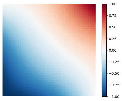
Approximate the solution for \(u_x(0,y) = 0\), \(u(1,y) = -\cos(\pi y)\), \(u(x,0) = -1\) and \(u(x,1) = 1\).

f0 = lambda y: 0.
f1 = lambda y: -np.cos(np.pi*y)
g0 = lambda x: -1.
g1 = lambda x: 1.
U = laplace('N',f0,'D',f1,'D',g0,'D',g1)
plot_laplace(U)

Found approximation U with dUk = 9.95972846485963e-06 after k = 1227 iterations.