Heat Equation

import numpy as np
import matplotlib.pyplot as plt

The heat equation (or diffusion equation) is given by

\[ \frac{\partial u}{\partial t} = \alpha^2 \frac{\partial^2 u}{\partial x^2} \ , \ \ 0 \leq x \leq L \ , \ \ t \geq 0 \ , \ \ \alpha \in \mathbb{R} \]

Initial and Boundary Conditions

The initial condition is a function \(f(x)\) which determines the solution \(u(x,0) = f(x)\) at time \(t=0\).

Dirichlet boundary conditions specify the values of the solution at the endpoints:

\[ u(0,t) = T_0 \ \ \ \text{and} \ \ \ u(L,t) = T_L \]

Neumann boundary conditions specify the values of the derivative of the solution at the endpoints:

\[ u_x(0,t) = Q_0 \ \ \ \text{and} \ \ \ u_x(L,t) = Q_L \]

When one endpoint is a Dirichlet boundary condition and the other is a Neumann boundary condition then we call them mixed boundary conditions. For example:

\[ u(0,t) = T_0 \ \ \ \text{and} \ \ \ u_x(L,t) = Q_L \]

Discretization

Choose the number of steps \(N\) in the \(x\) direction and the number of steps \(K\) in the \(t\) direction. These choices determine the step sizes \(\Delta x\) and \(\Delta t\), and create a grid of points:

\[\begin{split} \begin{align} x_n &= n \Delta x \ , \ \ n = 0,1, \dots, N \ , \ \ \Delta x = \frac{L}{N} \\ t_k &= k \Delta t \ , \ \ k = 0,1, \dots, K \ , \ \ \Delta t = \frac{t_f}{K} \end{align} \end{split}\]

Here we have chosen some final time value \(t_f\) so that the domain of the solution \(u(x,t)\) is a finite rectangle \([0,L] \times [0,t_f]\). The goal of a finite difference method is to compute the matrix

\[ U = [u_{n,k}] \]

which gives approximations of the solution \(u(x,t)\) at the grid points:

\[ u_{n,k} \approx u(x_n,t_k) = u(n \Delta x,k \Delta t) \]

where \(x_0 = 0\), \(x_N = L\), \(t_0 = 0\) and \(t_K = t_f\).

Forward Time Central Space

Apply the forward difference formula for \(u_t\) at position \(x_n\) and time \(t_k\)

\[\begin{split} \begin{align*} u_t(x_n,t_k) &= \frac{u(x_n,t_{k+1}) - u(x_n,t_k)}{\Delta t} + O(\Delta t) \\ &= \frac{u_{n,k+1} - u_{n,k}}{\Delta t} + O(\Delta t) \end{align*} \end{split}\]

Apply the central difference formula for \(u_{xx}\) at position \(x_n\) and time \(t_k\)

\[\begin{split} \begin{align*} u_{xx}(x_n,t_k) &= \frac{u(x_{n+1},t_k) - 2u(x_n,t_k) + u(x_{n-1},t_k)}{(\Delta x)^2} + O \left( (\Delta x)^2 \right) \\ &= \frac{u_{n+1,k} - 2u_{n,k} + u_{n-1,k}}{(\Delta x)^2} + O \left( (\Delta x)^2 \right) \end{align*} \end{split}\]

Plug the formulas into the heat equation at position \(x_n\) and time \(t_k\)

\[\begin{split} \begin{align*} u_t(x_n,t_k) &= \alpha^2 u_{xx}(x_n,t_k) \\ \frac{u_{n,k+1} - u_{n,k}}{\Delta t} &= \alpha^2 \left( \frac{u_{n+1,k} - 2u_{n,k} + u_{n-1,k}}{(\Delta x)^2} \right) \end{align*} \end{split}\]

Rearrange to solve for \(u_{n,k+1}\)

\[ u_{n,k+1} = r u_{n-1,k} + (1 - 2r) u_{n,k} + r u_{n+1,k} \ \ , \ \ r = \frac{\alpha^2 \Delta t}{(\Delta x)^2} \]

This is the forward-time-central-space (FTCS) finite difference method for the heat equation.

FTCS with Dirichlet BCs

Matrix Equations

Consider Dirichlet boundary conditions \(u(0,t) = T_0\) and \(u(L,t)\). Let \(u_{0,k} = T_0\) and \(u_{N,k} = T_L\) for all \(k\) and write out the FTCS equations for \(n=1,\dots,N-1\) along with the boundary conditions \(u_{0,k+1} = u_{0,k}\) and \(u_{N,k+1} = u_{N,k}\):

\[\begin{split} \begin{array}{cccccccccccccc} u_{0,k+1} & = & u_{0,k} & & & & & & & & & & \\ u_{1,k+1} & = & r u_{0,k} & + & (1 - 2r) u_{1,k} & + & r u_{2,k} & & & & & & \\ u_{2,k+1} & = & & & r u_{1,k} & + & (1 - 2r) u_{2,k} & + & r u_{3,k} & & & & \\ & \vdots & & & & & & \ddots & & & & & \\ u_{N-2,k+1} & = & & & & & r u_{N-3,k} & + & (1 - 2r) u_{N-2,k} & + & r u_{N-1,k} & & \\ u_{N-1,k+1} & = & & & & & & & r u_{N-2,k} & + & (1 - 2r) u_{N-1,k} & + & r u_{N,k} \\ u_{N,k+1} & = & & & & & & & & & & & u_{N,k} \end{array} \end{split}\]

These finite difference equations show us that approximations at time \(t_{k+1}\) are given by matrix multiplication of the vector of approximations at time \(t_k\). Therefore we can write the FTCS method as an iterative matrix formula.

\[ \boldsymbol{u}_{k+1} = A \boldsymbol{u}_k \]

where

\[\begin{split} A = \left[ \begin{array}{ccccccc} 1 & & & & & \\ r & 1 - 2r & r & & & & \\ & r & 1 - 2r & r & & & \\ & & & \ddots & & & \\ & & & r & 1 - 2r & r & \\ & & & & r & 1 - 2r & r \\ & & & & & & 1 \end{array} \right] \end{split}\]

\[\begin{split} \boldsymbol{u}_k = \begin{bmatrix} u_{0,k} \\ u_{1,k} \\ \vdots \\ u_{N-1,k} \\ u_{N,k} \end{bmatrix} \hspace{20mm} r = \frac{\alpha^2 \Delta t}{(\Delta x)^2} \end{split}\]

The algorithm produces the matrix of approximations

\[\begin{split} U = [u_{n,k}] = \begin{bmatrix} & & & \\ \boldsymbol{u}_0 & \boldsymbol{u}_1 & \cdots & \boldsymbol{u}_M \\ & & & \end{bmatrix} \ \ , \ \ \ u_{n,k} \approx u(x_n,t_k) \end{split}\]

starting from the initial condition

\[\begin{split} \boldsymbol{u}_0 = \begin{bmatrix} u_{0,0} \\ u_{1,0} \\ \vdots \\ u_{N,0} \end{bmatrix} = \begin{bmatrix} f(x_0) \\ f(x_1) \\ \vdots \\ f(x_N) \end{bmatrix} \end{split}\]

Note that we can create the matrix \(A\) with a for loop. For example:

N = 5
r = 0.01

A = np.zeros((N+1,N+1))
A[0,0] = 1
A[N,N] = 1
for n in range(1,N):
    A[n,n-1] = r
    A[n,n] = 1 - 2*r
    A[n,n+1] = r

print(A)

[[1.   0.   0.   0.   0.   0.  ]
 [0.01 0.98 0.01 0.   0.   0.  ]
 [0.   0.01 0.98 0.01 0.   0.  ]
 [0.   0.   0.01 0.98 0.01 0.  ]
 [0.   0.   0.   0.01 0.98 0.01]
 [0.   0.   0.   0.   0.   1.  ]]

Implementation

The function heatFTCSD takes input parameters alpha, L, f, T0, TL, tf, N and K, and returns the matrix U of approximations where:

• alpha is the diffusion coefficient in the heat equation \(u_t = \alpha^2 u_{xx}\)

• L is the length of the interval \(0 \leq x \leq L\)

• f is a Python function whcih represents the initial condition \(u(x,0) = f(x)\)

• T0 is the boundary condition \(u(0,t) = T_0\)

• TL is the boundary condition \(u(L,t) = T_L\)

• tf is the length of the interval \(0 \leq t \leq t_f\)

• N is the number of steps in the \(x\)-direction of the discretization

• K is the number of steps in the \(t\)-direction of the discretization

• U is the matrix \(U = [u_{n,k}]\) of size \((N+1) \times (K+1)\) of approximations \(u_{n,k} \approx u(x_n,t_k)\)

def heatFTCSD(alpha,L,f,T0,TL,tf,N,K):
    dx = L/N
    dt = tf/K
    x = np.linspace(0,L,N+1)
    U = np.zeros((N+1,K+1))
    U[:,0] = f(x)
    U[0,0] = T0
    U[N,0] = TL
    r = alpha*dt/dx**2
    A = np.zeros((N+1,N+1))
    A[0,0] = 1
    A[N,N] = 1
    for n in range(1,N):
        A[n,n-1] = r
        A[n,n] = 1 - 2*r
        A[n,n+1] = r
    for k in range(K):
        U[:,k+1] = A@U[:,k]
    return U

Example

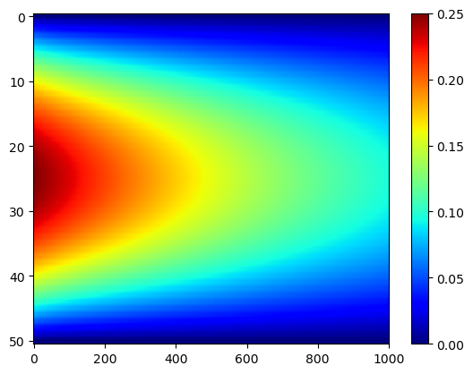
Consider \(\alpha = 0.1\), \(L = 1\), \(f(x) = x(1-x)\), \(T_0 = 0\), \(T_L\) and \(t_f = 1\).

alpha = 0.1
L = 1
f = lambda x: x*(1 - x)
T0 = 0
TL = 0
tf = 1
N = 50
K = 1000

U = heatFTCSD(alpha,L,f,T0,TL,tf,N,K)

plt.imshow(U,aspect='auto',cmap='jet')
plt.colorbar()
plt.show()

FTCS with Neumann BCs

Matrix Equations

Consider Neumann boundary conditions \(u_x(0,t) = Q_0\) and \(u_x(L,t) = Q_L\). The FTCS finite difference equation at \(n=0\) yields

\[ u_{0,k+1} = r u_{-1,k} + (1 - 2r) u_{0,k} + r u_{1,k} \]

with the “ghost value” \(u_{-1,k}\). Use the central difference formula for \(u_x(0,t_k) = Q_0\)

\[ Q_0 = \frac{u_{1,k} - u_{-1,k}}{2 \Delta x} \]

Rearrange for \(u_{-1,k}\)

\[ u_{-1,k} = u_{1,k} - 2 \Delta x Q_0 \]

and substitute into the FTCS equation

\[ u_{0,k+1} = (1 - 2r) u_{0,k} + 2 r u_{1,k} - \frac{2 \alpha^2 \Delta t Q_0}{\Delta x} \]

Similarly, the boundary condition \(u_x(L,t) = Q_L\) yields the equation

\[ u_{N,k+1} = 2r u_{N-1,k} + (1 - 2r)u_{N,k} + \frac{2 \alpha^2 \Delta t Q_L}{\Delta x} \]

Write out the FTCS equations for \(n=1,\dots,N-1\) along with the boundary conditions:

\[\begin{split} \begin{array}{ccccccccc} u_{0,k+1} & = & (1 - 2r)u_{0,k} & + & 2r u_{1,k} & & & - & \frac{2 \alpha^2 \Delta t Q_0}{\Delta x} \\ u_{1,k+1} & = & r u_{0,k} & + & (1 - 2r) u_{1,k} & + & r u_{2,k} & & \\ & \vdots & & \vdots & & \vdots & & & \\ u_{N-1,k+1} & = & r u_{N-2,k} & + & (1 - 2r) u_{N-1,k} & + & r u_{N,k} & & \\ u_{N,k+1} & = & & & 2r u_{N-1,k} & + & (1 - 2r)u_{N,k} & + & \frac{2 \alpha^2 \Delta t Q_L}{\Delta x} \end{array} \end{split}\]

These finite difference equations show us that approximations at time \(t_{k+1}\) are given by matrix multiplication of the vector of approximations at time \(t_k\). Therefore we can write the FTCS method as an iterative matrix formula.

\[ \boldsymbol{u}_{k+1} = A \boldsymbol{u}_k + \boldsymbol{q} \]

where

\[\begin{split} A = \left[ \begin{array}{ccccccc} 1 - 2r & 2r & & & & \\ r & 1 - 2r & r & & & & \\ & r & 1 - 2r & r & & & \\ & & & \ddots & & & \\ & & & r & 1 - 2r & r & \\ & & & & r & 1 - 2r & r \\ & & & & & 2r & 1 - 2r \end{array} \right] \end{split}\]

\[\begin{split} \boldsymbol{u}_k = \begin{bmatrix} u_{0,k} \\ u_{1,k} \\ \vdots \\ u_{N-1,k} \\ u_{N,k} \end{bmatrix} \hspace{20mm} \boldsymbol{q} = \frac{2 \alpha^2 \Delta t}{\Delta x} \begin{bmatrix} -Q_0 \\ 0 \\ \vdots \\ 0 \\ Q_L \end{bmatrix} \hspace{20mm} r = \frac{\alpha^2 \Delta t}{(\Delta x)^2} \end{split}\]

The algorithm produces the matrix of approximations

\[\begin{split} U = [u_{n,k}] = \begin{bmatrix} & & & \\ \boldsymbol{u}_0 & \boldsymbol{u}_1 & \cdots & \boldsymbol{u}_M \\ & & & \end{bmatrix} \ \ , \ \ \ u_{n,k} \approx u(x_n,t_k) \end{split}\]

starting from the initial condition

\[\begin{split} \boldsymbol{u}_0 = \begin{bmatrix} u_{0,0} \\ u_{1,0} \\ \vdots \\ u_{N,0} \end{bmatrix} = \begin{bmatrix} f(x_0) \\ f(x_1) \\ \vdots \\ f(x_N) \end{bmatrix} \end{split}\]

Implementation

The function heatFTCSN takes input parameters alpha, L, f, Q0, QL, tf, N and K, and returns the matrix U of approximations where:

• alpha is the diffusion coefficient in the heat equation \(u_t = \alpha^2 u_{xx}\)

• L is the length of the interval \(0 \leq x \leq L\)

• f is a Python function whcih represents the initial condition \(u(x,0) = f(x)\)

• Q0 is the boundary condition \(u_x(0,t) = Q_0\)

• QL is the boundary condition \(u_x(L,t) = Q_L\)

• tf is the length of the interval \(0 \leq t \leq t_f\)

• N is the number of steps in the \(x\)-direction of the discretization

• K is the number of steps in the \(t\)-direction of the discretization

• U is the matrix \(U = [u_{n,k}]\) of size \((N+1) \times (K+1)\) of approximations \(u_{n,k} \approx u(x_n,t_k)\)

def heatFTCSN(alpha,L,f,Q0,QL,tf,N,K):
    dx = L/N
    dt = tf/K
    x = np.linspace(0,L,N+1)
    U = np.zeros((N+1,K+1))
    U[:,0] = f(x)
    r = alpha*dt/dx**2
    A = np.zeros((N+1,N+1))
    A[0,0] = 1 - 2*r
    A[0,1] = 2*r
    A[N,N] = 1 - 2*r
    A[N,N-1] = 2*r
    for n in range(1,N):
        A[n,n-1] = r
        A[n,n] = 1 - 2*r
        A[n,n+1] = r
    q = np.zeros(N+1)
    q[0] = -2*alpha**2*dt/dx*Q0
    q[N] = 2*alpha**2*dt/dx*QL
    for k in range(K):
        U[:,k+1] = A@U[:,k] + q
    return U

Example

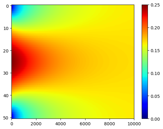
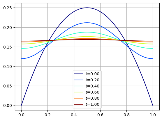
Consider \(\alpha = 0.1\), \(L = 1\), \(f(x) = x(1-x)\), \(Q_0=Q_L=0\) and \(t_f = 1\).

alpha = 0.1
L = 1
f = lambda x: x*(1 - x)
Q0 = 0
QL = 0
tf = 1
N = 50
K = 10000

U = heatFTCSN(alpha,L,f,Q0,QL,tf,N,K)

plt.imshow(U,aspect='auto',cmap='jet'), plt.colorbar()
plt.show()

nsteps = 5
tstep = K//nsteps
x = np.linspace(0,L,N+1)
for k in range(nsteps+1):
    t = k*tstep*tf/K
    plt.plot(x,U[:,k*tstep],color=plt.cm.jet(t),label='t={:.2f}'.format(t))
plt.legend()
plt.grid(True)
plt.show()

FTCS with Mixed BCs

Combine both functions heatFTCSD and heatFTCSN into a single function heat which takes input parameters alpha, L, f, BCtype0, BC0, BCtypeL, BCL, tf, N and K, and returns the matrix U of approximations where:

• alpha is the diffusion coefficient in the heat equation \(u_t = \alpha^2 u_{xx}\)

• L is the length of the interval \(0 \leq x \leq L\)

• f is a Python function which represents the initial condition \(u(x,0) = f(x)\)

• BCtype0 is the type of boundary condition at \(x=0\) ('D' for Dirichlet or 'N' for Neumann)

• BC0 is the value of the boundary condition at \(x=0\)

• BCtypeL is the type of boundary condition at \(x=L\) ('D' for Dirichlet or 'N' for Neumann)

• BCL is the value of the boundary condition at \(x=L\)

• tf is the length of the interval \(0 \leq t \leq t_f\)

• N is the number of steps in the \(x\)-direction of the discretization

• K is the number of steps in the \(t\)-direction of the discretization

• U is the matrix \(U = [u_{n,k}]\) of size \((N+1) \times (K+1)\) of approximations \(u_{n,k} \approx u(x_n,t_k)\)

def heat(alpha,L,f,BCtype0,BC0,BCtypeL,BCL,tf,N,K):
    dx = L/N
    dt = tf/K
    r = alpha*dt/dx**2
    x = np.linspace(0,L,N+1)
    U = np.zeros((N+1,K+1))
    U[:,0] = f(x)
    A = np.zeros((N+1,N+1))
    q = np.zeros(N+1)
    
    if (BCtype0 not in ['D','N']) or (BCtypeL not in ['D','N']):
        raise Exception("Expecting boundary conditions of type 'D' or 'N'.")
    if BCtype0 == 'D':
        U[0,0] = BC0
        A[0,0] = 1
    if BCtype0 == 'N':
        A[0,0] = 1 - 2*r
        A[0,1] = 2*r
        q[0] = -2*alpha**2*dt/dx*BC0
    if BCtypeL == 'D':
        U[N,0] = BCL
        A[N,N] = 1
    if BCtypeL == 'N':
        A[N,N] = 1 - 2*r
        A[N,N-1] = 2*r
        q[N] = 2*alpha**2*dt/dx*BCL
    
    for n in range(1,N):
        A[n,n-1] = r
        A[n,n] = 1 - 2*r
        A[n,n+1] = r
        
    for k in range(K):
        U[:,k+1] = A@U[:,k] + q
        
    return U

Consider \(\alpha = 0.1\), \(L = 1\), \(f(x) = x(1-x)\), \(u_x(0,t) = u_x(L,t) = 0\) and \(t_f = 1\).

alpha = 0.1
L = 1
f = lambda x: x*(1 - x)
BCtype0 = 'N'
Q0 = 0
BCtypeL = 'N'
QL = 0
tf = 1
N = 50
K = 10000

U = heat(alpha,L,f,BCtype0,Q0,BCtypeL,QL,tf,N,K)

plt.imshow(U,aspect='auto',cmap='jet'), plt.colorbar()
plt.show()

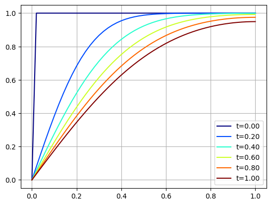
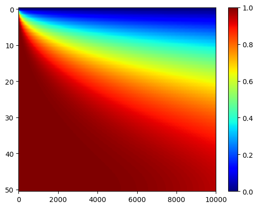
Consider \(\alpha = 0.1\), \(L = 1\), \(f(x) = 1\), \(u(0,t)=u_x(L,t)=0\) and \(t_f = 1\).

alpha = 0.1
L = 1
f = lambda x: np.ones_like(x)
BCtype0 = 'D'
T0 = 0
BCtypeL = 'N'
QL = 0
tf = 1
N = 50
K = 10000

U = heat(alpha,L,f,BCtype0,T0,BCtypeL,QL,tf,N,K)

plt.imshow(U,aspect='auto',cmap='jet'), plt.colorbar()
plt.show()

nsteps = 5
tstep = K//nsteps
x = np.linspace(0,L,N+1)
for k in range(nsteps+1):
    t = k*tstep*tf/K
    plt.plot(x,U[:,k*tstep],color=plt.cm.jet(t),label='t={:.2f}'.format(t))
plt.legend()
plt.grid(True)
plt.show()