Numerical Solutions with odeint

Most differential equations cannot be solved analytically in terms of elementary functions. So what do we do? We can always approximate! The function scipy.integrate.odeint approximates solutions of first order equations using highly accurate and optimized numerical methods. Our goal is to learn how to use odeint and how to interpret the output.

import numpy as np
import matplotlib.pyplot as plt
import scipy.integrate as spi

Basic Procedure

The function scipy.integrate.odeint approximates the solution of a first order differential equation with an initial condition:

\[ y' = f(y,t) \ , \ \ y(t_0) = y_0 \]

The function scipy.integrate.odeint takes input parameters f, y0 and t where:

• f is a Python function which represents the right hand side of the equation \(y' = f(y,t)\)

• y0 is the initial value \(y(t_0) = y_0\)

• t is a NumPy array of \(t\) values such that the first entry is \(t_0\)

The fuction scipy.integrate.odeint returns a NumPy array y such that:

• the length of y is equal to the length of t

• the first value y[0] is the initial value \(y(t_0) = y_0\)

• the value y[n] at index \(n\) is an approximation of the solution \(y(t_n)\) at time \(t_n\)

• the value \(t_n\) is the entry t[n] at index \(n\) in the input array t

Given a differential equation with initial value, it is up to us to construct the input vector t. We need to choose a final value \(t_f\) and the number of values in the input vector t.

Examples

Example: \(y' = -2y^2t\)

Approximate the unique solution of the equation

\[ y' = -2y^2 t \ , \ \ y(0)=1 \]

over the interval \([0,5]\) and compare to the exact solution

\[ y(t) = \frac{1}{t^2 + 1} \]

Define the function f which represents the right hand side of the equation:

f = lambda y,t: -2*y**2*t

Plug in some values \(y\) and \(t\) to see that it simply returns the value \(-2y^2t\):

f(1,2)

-4

f(-1,1/2)

-1.0

Define the initial value:

y0 = 1

Construct a NumPy array of \(t\) values from \(t_0 = 0\) to \(t_f = 5\). The number of points in the array is our decision. The number of points does not change the accuracy of the results. It only changes the number of \(y\) values in the output and we need enough to plot the approximation smoothly. Let’s choose \(N=51\) values so that the step size between \(t\) values is 0.1.

t0 = 0; tf = 5; N = 51;
t = np.linspace(t0,tf,N)

Take a look at the first 5 entries of t:

t[:5]

array([0. , 0.1, 0.2, 0.3, 0.4])

And the last 5 entries:

t[-5:]

array([4.6, 4.7, 4.8, 4.9, 5. ])

Compute the approximations using odeint:

y = spi.odeint(f,y0,t)

Check the length of the NumPy array y:

len(y)

51

It’s the same as the length of t:

len(t)

51

Look at the first 5 entries of y:

y[:5]

array([[1.        ],
       [0.99009914],
       [0.96153854],
       [0.91743128],
       [0.86206907]])

The first value is the initial value \(y(0)=1\) and the approximations of the values \(y(t_n)\) are decreasing. Let’s plot the approximation with the exact solution.

plt.plot(t,y,'.',label='odeint')
T = np.linspace(t0,tf,200)
Y = 1/(T**2 + 1)
plt.plot(T,Y,label='Exact')
plt.legend()
plt.show()

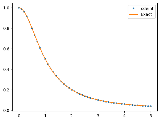
The approximation is almost indistinguishable from the exact solution!

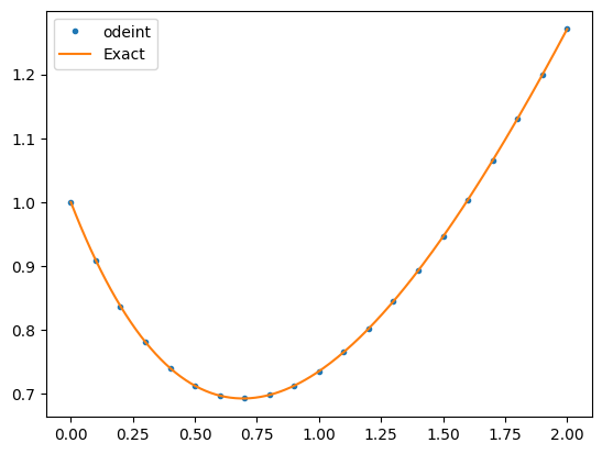
Example: \(y' = y - t\)

Approximate the unique solution of the equation

\[ y' = t - y \ , \ \ y(0) = 1 \]

over the interval \([0,2]\) and compare to the exact solution

\[ y(t) = 2e^{-t} + t - 1 \]

f = lambda y,t: t - y
y0 = 1
t0 = 0; tf = 2; N = 21;
t = np.linspace(t0,tf,N)
y = spi.odeint(f,y0,t)
plt.plot(t,y,'.',label='odeint')
T = np.linspace(t0,tf,200)
Y = 2*np.exp(-T) + T - 1
plt.plot(T,Y,label='Exact')
plt.legend()
plt.show()

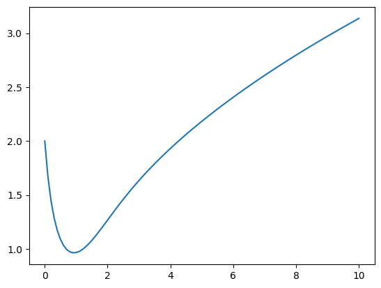
Example: \(y' = t - y^2\)

Approximate the unique solution of the equation

\[ y' = t - y^2 \ , \ \ y(0) = 2 \]

This is a nonlinear, nonseparable equation therefore we do not have an analytical method to find the exact solution. Use odeint to approximate the solution over the interval \([0,10]\).

f = lambda y,t: t - y**2
y0 = 2
t0 = 0; tf = 10; N = 101;
t = np.linspace(t0,tf,N)
y = spi.odeint(f,y0,t)
plt.plot(t,y)
plt.show()

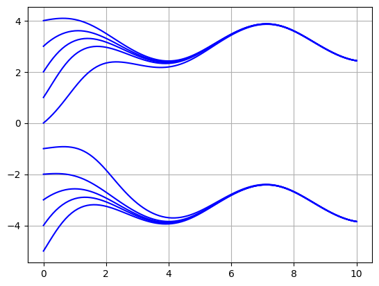
Example: \(y' = \cos(t) + \sin(y)\)

Approximate solutions of the equation

\[ y' = \cos(t) + \sin(y) \]

This is a nonlinear, nonseparable equation therefore we do not have an analytical method to find the exact solution. Use odeint to approximate the solution over the interval \([0,10]\) for several different initial conditions.

f = lambda y,t: np.cos(t) + np.sin(y)
t0 = 0; tf = 10; N = 101;
t = np.linspace(t0,tf,N)
for y0 in range(-5,5):
    y = spi.odeint(f,y0,t)
    plt.plot(t,y,'b')
plt.grid(True)
plt.show()