Linear Transformations

import numpy as np
import scipy.linalg as la
import matplotlib.pyplot as plt

Matrix Multiplication

Let’s create an asymmetrical figure in the xy-plane by defining lists of \(x\) and \(y\) coordinates.

x = [0.,-1.,-2.,0.,2.,1.,0.,1.]
y = [0.,2.,0.,-2.,0.,2.,0.,0.]
plt.plot(x,y,'.-'), plt.grid(True), plt.axis('equal')
plt.show()

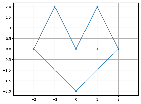
Note that we use the command plt.grid(True) to include a grid in the figure and plt.axis('equal') plots the figure with equal scaling in the \(x\) and \(y\) directions.

Stack the vectors of \(x\) and \(y\) coordinates to create a matrix \(X\). The columns of \(X\) are the coordinates of the points defining the vertices of the figure above. The row at index 0 are the \(x\)-coordinates and the row at index 1 are the \(y\)-coordinates.

X = np.row_stack([x,y])
print(X)

[[ 0. -1. -2.  0.  2.  1.  0.  1.]
 [ 0.  2.  0. -2.  0.  2.  0.  0.]]

/var/folders/2h/25vcwmr52mvfqs1h92028rph0000gn/T/ipykernel_33158/4224013073.py:1: DeprecationWarning: `row_stack` alias is deprecated. Use `np.vstack` directly.
  X = np.row_stack([x,y])

plt.plot(X[0,:],X[1,:],'.-'), plt.grid(True), plt.axis('equal')
plt.show()

Any linear transformation of \(\mathbb{R}^2\) can be written as a 2 by 2 matrix with respect to the standard basis. Therefore we can apply to the figure above a linear transformation given by matrix \(A\) by computing matrix multiplication:

\[\begin{split} AX = A \begin{bmatrix} x_0 & x_1 & \cdots & x_N \\ y_0 & y_1 & \cdots & y_N \end{bmatrix} = \begin{bmatrix} A \begin{bmatrix} x_0 \\ y_0 \end{bmatrix} & A \begin{bmatrix} x_1 \\ y_1 \end{bmatrix} & \cdots & A \begin{bmatrix} x_N \\ y_N \end{bmatrix} \end{bmatrix} \end{split}\]

where column at index \(k\) corresponds to the point \((x_k,y_k) \in \mathbf{R}^2\). In other words, the column at index \(k\) in the product \(AX\) are the coordinates of the transformed point \(A \begin{bmatrix} x_k \\ y_k \end{bmatrix}\).

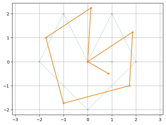
Rotation Matrix

A rotation matrix is given by

\[\begin{split} R_{\theta} = \begin{bmatrix} \cos(\theta) & \sin(\theta) \\ -\sin(\theta) & \cos(\theta) \end{bmatrix} \end{split}\]

The linear transformation corresponding to \(R_{\theta}\) is rotation about the origin clockwise by \(\theta\) radians.

theta = np.pi/6
R = np.array([[np.cos(theta),np.sin(theta)],[-np.sin(theta),np.cos(theta)]])
RX = R@X

plt.plot(X[0,:],X[1,:],'.-',alpha=0.2)
plt.plot(RX[0,:],RX[1,:],'.-'), plt.axis('equal'), plt.grid(True)
plt.show()

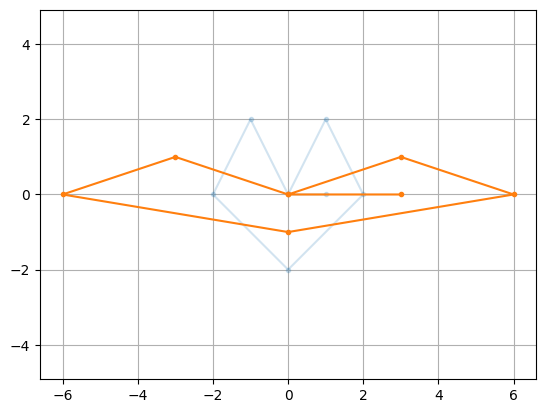
Scaling Matrix

A scaling matrix is given by

\[\begin{split} C_{a,b} = \begin{bmatrix} a & 0 \\ 0 & b \end{bmatrix} \end{split}\]

The linear transformation corresponding to \(C_{a,b}\) is scaling by \(a\) is the \(x\)-direction and scaling by \(b\) in the \(y\)-direction.

a = 3; b = 1/2;
C = np.diag([a,b])
CX = C@X

plt.plot(X[0,:],X[1,:],'.-',alpha=0.2)
plt.plot(CX[0,:],CX[1,:],'.-'), plt.axis('equal'), plt.grid(True)
plt.show()

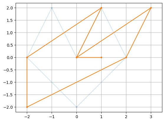
Shear Matrix

A shear matrix is given by

\[\begin{split} S_u = \begin{bmatrix} 1 & u \\ 0 & 1 \end{bmatrix} \end{split}\]

The linear transformation corresponding to \(S_u\) is shear by factor \(u\) in the \(x\)-direction.

u = 1
S = np.array([[1,u],[0,1]])
SX = S@X

plt.plot(X[0,:],X[1,:],'.-',alpha=0.2)
plt.plot(SX[0,:],SX[1,:],'.-'), plt.axis('equal'), plt.grid(True)
plt.show()

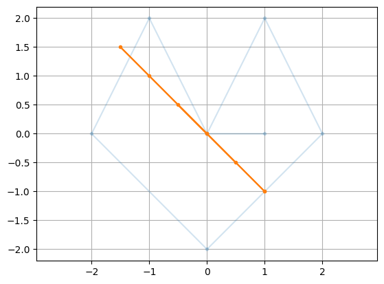
Projection Matrix

The matrix which projects onto the line at angle \(\theta\) with the \(x\)-axis is given by

\[\begin{split} P_{\theta} = \begin{bmatrix} \cos^2 \theta & \cos \theta \sin \theta \\ \cos \theta \sin \theta & \sin^2 \theta \end{bmatrix} \end{split}\]

theta = -np.pi/4
P = np.array([[np.cos(theta)**2,np.cos(theta)*np.sin(theta)],
              [np.cos(theta)*np.sin(theta),np.sin(theta)**2]])
PX = P@X

plt.plot(X[0,:],X[1,:],'.-',alpha=0.2)
plt.plot(PX[0,:],PX[1,:],'.-'), plt.axis('equal'), plt.grid(True)
plt.show()

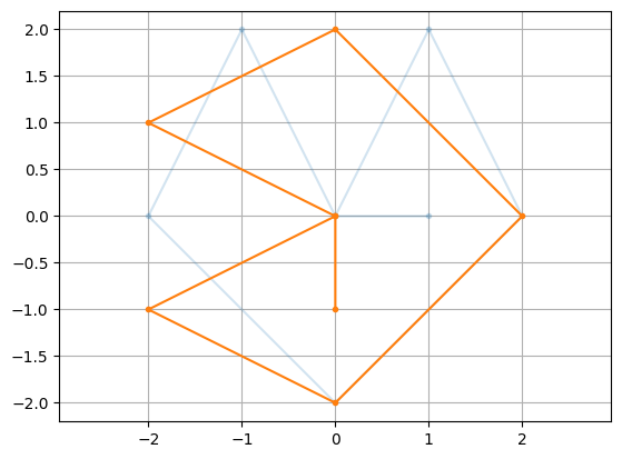
Reflection Matrix

The matrix which refelcts through the line at angle \(\theta\) with the \(x\)-axis is given by

\[\begin{split} F_{\theta} = \begin{bmatrix} \cos 2\theta & \sin 2\theta \\ \sin 2\theta & -\cos 2 \theta \end{bmatrix} \end{split}\]

theta = -np.pi/4
F = np.array([[np.cos(2*theta),np.sin(2*theta)],
              [np.sin(2*theta),-np.cos(2*theta)]])
FX = F@X

plt.plot(X[0,:],X[1,:],'.-',alpha=0.2)
plt.plot(FX[0,:],FX[1,:],'.-'), plt.axis('equal'), plt.grid(True)
plt.show()