Numerical Integration

import numpy as np
import matplotlib.pyplot as plt

Visualizing Riemann Sums

The definite integral \(\int_a^b f(x) \, dx\) is the (net) area under the curve \(y=f(x)\). Approximate the area under the curve by the sum of areas of rectangles. In particular, choose an integer \(N\) and define

\[ x_k = a + k \Delta x \ \ \ , \ \ \Delta x = \frac{b - a}{N} \ \ \ , \ \ k=0,1,\dots,N \]

The values \(x_0,x_1,\dots,x_N\) define a partition of the interval \([a,b]\) with \(N\) subintervals. Note that \(x_0 = a\) and \(x_N = b\). Define a rectangle over each subinterval \([x_{k-1},x_k]\), \(k=1,\dots,N\), with height using the right endpoint \(f(x_k)\) or the left endpoint \(f(x_{k-1})\). Using the right endpoint we get the right Riemann sum

\[ R = \sum_{k=1}^N f(x_k) \Delta x = \left( \frac{b-a}{N} \right) \sum_{k=1}^N f(x_k) \]

Using the left endpoint we get the left Riemann sum

\[ L = \sum_{k=1}^N f(x_{k-1}) \Delta x = \left( \frac{b-a}{N} \right) \sum_{k=1}^N f(x_{k-1}) \]

Each Riemann sum is an approximation of the definite integral \(\int_a^b f(x) \, dx\). The definite integral is equal to the limit

\[ \int_a^b f(x) \, dx = \lim_{N \to \infty} \sum_{k=1}^N f(x_k^*) \Delta x \]

where \(x_k^*\) is any value in the interval \([x_{k-1},x_k]\).

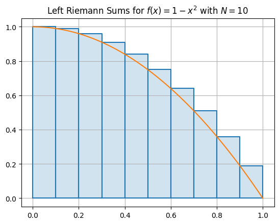
Let’s visualize the area under curve approximated by rectangles. Consider the function \(f(x) = 1-x^2\) over the interval \([0,1]\) and plot rectangles for the left Riemann sum.

# Define the function
f = lambda x: 1 - x**2

# Define the partition of [a,b] consisting of N subintervals of equal length
a = 0; b = 1; N = 10; dx = (b - a)/N;
x = np.linspace(a,b,N+1)

# Compute the y values at each point x[k] in the partition
y = f(x)

# Plot a rectangle for each subinterval [x[k-1],x[k]]
for k in range(1,N+1):
    
    # Plot a filled rectangle with base from x[k-1] to x[k] and height y[k-1]
    plt.fill([x[k-1],x[k-1],x[k],x[k]],[0,y[k-1],y[k-1],0],'C0',alpha=0.2)
    
    # Plot the outline of the rectangle with base from x[k-1] to x[k] and height y[k-1]
    plt.plot([x[k-1],x[k-1],x[k],x[k],x[k-1]],[0,y[k-1],y[k-1],0,0],'C0')

# Compute many values y = f(x) so that we can plot y = f(x) smoothly
X = np.linspace(a,b,(b-a)*100)
Y = f(X)
plt.plot(X,Y,'C1')

# Add style to the figure
plt.grid(True)
plt.title('Left Riemann Sums for $f(x) = 1-x^2$ with $N={}$'.format(N))
plt.show()

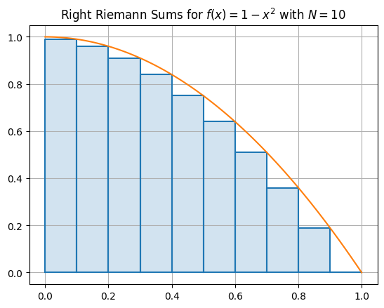
Let’s do the same example but for right Riemann sums.

# Define the function
f = lambda x: 1 - x**2

# Define the partition of [a,b] consisting of N subintervals of equal length
a = 0; b = 1; N = 10; dx = (b - a)/N;
x = np.linspace(a,b,N+1)

# Compute the y values at each point x[k] in the partition
y = f(x)

# Plot a rectangle for each subinterval [x[k-1],x[k]]
for k in range(1,N+1):
    
    # Plot a filled rectangle with base from x[k-1] to x[k] and height y[k]
    plt.fill([x[k-1],x[k-1],x[k],x[k]],[0,y[k],y[k],0],'C0',alpha=0.2)
    
    # Plot the outline of the rectangle with base from x[k-1] to x[k] and height y[k]
    plt.plot([x[k-1],x[k-1],x[k],x[k],x[k-1]],[0,y[k],y[k],0,0],'C0')

# Compute many values y = f(x) so that we can plot y = f(x) smoothly
X = np.linspace(a,b,(b-a)*100)
Y = f(X)
plt.plot(X,Y,'C1')

# Add style to the figure
plt.grid(True)
plt.title('Right Riemann Sums for $f(x) = 1-x^2$ with $N={}$'.format(N))
plt.show()

Computing Riemann Sums

The right Riemann for the definite integral \(\int_a^b f(x) dx\) is given by

\[ R = \left( \frac{b - a}{N} \right) \sum_{k=1}^N y_k \]

where \(y_k = f(x_k)\) is the value at the right endpoint of the interval \([x_{k-1},x_k]\) for each \(k=1,\dots,N\).

The procedure to compute the right Riemann sum is as follows:

1. Define the function \(y = f(x)\) and limits of integration \(a\) and \(b\)

2. Choose a value \(N\) and compute the value \(\Delta x = (b - a)/N\)

3. Use np.linspace to create the vector of \(x\) values in the partition

4. Use vectorization to compute the vector of \(y\) values

5. Compute the sum of the \(y\) values from index \(k=1\) to \(k=N\) and multiply by \(\Delta x\)

Let’s do the example from the previous exercise \(\int_0^1 (1 - x^2) \, dx\). We know the exact value is \(2/3\) and so we can compare our results. First, define the function \(f(x)\):

f = lambda x: 1 - x**2
a = 0
b = 1

Choose a value \(N\). This is entirely up to us. Higher value \(N\) gives a better approximation but requires more memory and time to compute the sum. Let’s start small and then increase it later.

N = 5
dx = (b - a)/N

Compute the vector \(\mathbf{x}\) given by the values \(x_k = a + k \Delta x\), \(k=0,1,\dots,N\). Note that there are \(N+1\) values in the vector \(\mathbf{x}\).

x = np.linspace(a,b,N+1)

Print the vector to verify:

print(x)

[0.  0.2 0.4 0.6 0.8 1. ]

Apply the function \(f(x)\) to the vector \(\mathbf{x}\). The result is the vector

\[ \mathbf{y} = f(\mathbf{x}) = \begin{bmatrix} f(x_0) & f(x_1) & \cdots & f(x_N) \end{bmatrix} \]

In other words, the value of \(\mathbf{y}\) at in dex \(k\) is \(y_k = f(x_k)\).

y = f(x)

Print the vector to verify:

print(y)

[1.   0.96 0.84 0.64 0.36 0.  ]

Select the values of y from index 1 to N using the command:

y[1:]

array([0.96, 0.84, 0.64, 0.36, 0.  ])

Approximate the integral using the right Riemann sums:

R = np.sum(y[1:])*(b - a)/N
print(R)

0.5599999999999998

Let’s put it all together in one cell and then increase \(N\) to get better approximations:

f = lambda x: 1 - x**2
a = 0; b = 1; N = 20; dx = (b - a)/N;
x = np.linspace(a,b,N+1)
y = f(x)
R = np.sum(y[1:])*(b - a)/N
print(R)

0.64125

The left Riemann for the definite integral \(\int_a^b f(x) dx\) is given by

\[ L = \left( \frac{b - a}{N} \right) \sum_{k=1}^N y_{k-1} \]

where \(y_{k-1} = f(x_{k-1})\) is the value at the left endpoint of the interval \([x_{k-1},x_k]\) for each \(k=1,\dots,N\).

Note that we can make the substitution in the index \(k - 1 \to k\) to rewrite the sum as

\[ L = \left( \frac{b - a}{N} \right) \sum_{k=0}^{N-1} y_k \]

The procedure to compute the left Riemann sum is exactly the same but this time we need to select the values of the vector y from index 0 to N-1.

f = lambda x: 1 - x**2
a = 0; b = 1; N = 5; dx = (b - a)/N;
x = np.linspace(a,b,N+1)
y = f(x)
print(y)

[1.   0.96 0.84 0.64 0.36 0.  ]

Select the values of y from index 0 to N-1 using the command:

y[:N]

array([1.  , 0.96, 0.84, 0.64, 0.36])

Approximate the integral using the left Riemann sums:

f = lambda x: 1 - x**2
a = 0; b = 1; N = 20; dx = (b - a)/N;
x = np.linspace(a,b,N+1)
y = f(x)
L = np.sum(y[:N])*(b - a)/N
print(L)

0.6912499999999999

We know that \(\int_0^1 (1 - x^2) \, dx = 2/3\) therefore the Riemann sums approach \(2/3\) as \(N \to \infty\).

Computing the Trapezoid Rule

The left and right Riemann sums are approximations of the definite integral \(\int_a^b f(x) \, dx\). The trapezoid rule is the average of the left and right Riemann sums

\[ T = \frac{L + R}{2} = \frac{1}{2} \left( \sum_{k=1}^N f(x_{k-1}) \Delta x + \sum_{k=1}^N f(x_k) \Delta x \right) = \left( \frac{b-a}{N} \right) \sum_{k=1}^N \left( \frac{f(x_{k-1}) + f(x_k)}{2} \right) \]

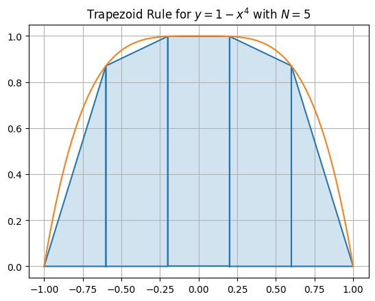
The trapezoid rule corresponds to the sum of the areas of the trapezoids below the curve on each subinterval.

For example, let’s plot the trapezoids for \(f(x) = 1-x^4\) in the interval \([-1,1]\) for \(N=5\).

f = lambda x: 1 - x**4
a = -1; b = 1; N = 5;
x = np.linspace(a,b,N+1)
y = f(x)

# Plot a rectangle for each subinterval [x[k-1],x[k]]
for k in range(1,N+1):
    
    # Plot a filled trapezoid with base from x[k-1] to x[k] and height y[k]
    plt.fill([x[k-1],x[k-1],x[k],x[k]],[0,y[k-1],y[k],0],'C0',alpha=0.2)
    
    # Plot the outline of the rectangle with base from x[k-1] to x[k] and height y[k]
    plt.plot([x[k-1],x[k-1],x[k],x[k],x[k-1]],[0,y[k-1],y[k],0,0],'C0')

# Compute many values y = f(x) so that we can plot y = f(x) smoothly
X = np.linspace(a,b,(b-a)*100)
Y = f(X)
plt.plot(X,Y,'C1')

# Add style to the figure
plt.grid(True)
plt.title('Trapezoid Rule for $y = 1-x^4$ with $N={}$'.format(N))
plt.show()

Let’s compute the average of the left and right Riemann sums:

f = lambda x: 1 - x**4
a = -1; b = 1; N = 100;
x = np.linspace(a,b,N+1)
y = f(x)
T = (b - a)/N*(np.sum(y[1:] + y[:N]))/2
print('T =',T)

T = 1.5997333440000003

The exact solution is \(\int_{-1}^1 (1 - x^4) \, dx = 8/5\) therefore \(T\) converges to \(1.6\) as \(N \to \infty\).

Visualizing Riemann Sums for Double Integrals

Let \(R\) be the region bounded between the curves \(y = B(x)\) and \(y = T(x)\) and \(a \leq x \leq b\). Let \(f(x,y)\) be an integrable function. The definite integral of \(f(x,y)\) over the region \(R\) is a limit of Riemann sums

\[ \iint_R f(x,y) \, dy dx = \int_a^b \int_{B(x)}^{T(x)} f(x,y) \, dy \, dx = \lim_{N \to \infty} \sum_{k=1}^N \left( \int_{B(x_k)}^{T(x_k)} f(x_k,y) dy \right) \Delta x = \lim_{N,M \to \infty} \sum_{k=1}^N \sum_{l=1}^M f(x_k,y_{kl}) \Delta y_k \Delta x \]

where

\[ x_k = a + k \Delta x \ \ \ , \ \ k = 1,\dots,N \ \ \ , \ \ \Delta x = \frac{b - a}{N} \]

and

\[ y_{kl} = B(x_k) + l \Delta y_k \ \ \ , \ \ k = 1,\dots,N \ \ \ , \ \ l = 1,\dots,M \ \ \ , \ \ \Delta y_k = \frac{T(x_k) - B(x_k)}{M} \]

Note that \(x_0=a\) and \(x_N=b\), and \(y_{k,0},y_{k,1},\dots,y_{k,M}\) is a partition of \([B(x_k),T(x_k)]\) for each \(k=1,\dots,N\).

What does any of this mean?!!!

Let’s plot all the points \((x_k,y_{kl}) \in \mathbb{R}^2\) for \(k=0,\dots,N\) and \(l=0,\dots,M\) for the area bounded by the curves \(T(x) = 1 + \sqrt{x}\) and \(B(x) = x^2\) for \(0 \leq x \leq 1\).

T = lambda x: 1 + np.sqrt(x)
B = lambda x: x**2

N = 20;
x = np.linspace(0,1,N+1)

for k in range(N+1):
    M = 10
    y = np.linspace(B(x[k]),T(x[k]),M+1)
    for l in range(M+1):
        plt.plot(x[k],y[l],'b.')

plt.plot(x,T(x),'r'), plt.plot(x,B(x),'g')
plt.grid(True)
plt.show()

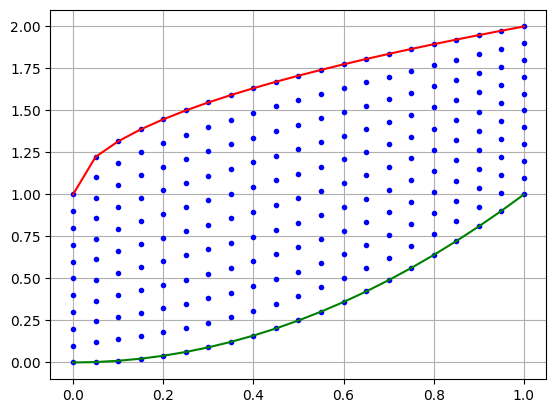
Now we can see all the points when we partition the \(x\)-interval \([a,b]\) and then partition each \(y\)-interval \([B(x_k),T(x_k)]\) for \(k=1,\dots,N\).

A Riemann sum is of the form

\[ \iint_R f(x,y) \, dy dx = \int_a^b \int_{B(x)}^{T(x)} f(x,y) \, dy \, dx \approx \sum_{k=1}^N \sum_{l=1}^M f(x_k^*,y_{kl}^*) \Delta y_k \Delta x \]

where \(x_k^* \in [x_{k-1},x_k]\) and \(y_{kl}^* \in [y_{k,l-1},y_{k,l}]\). The right Riemann sum is when we choose the right endpoints \(x_k^* = x_k\) and \(y_{kl}^* = y_{kl}\).

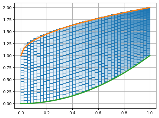
The value \(f(x_k^*,y_{kl}^*) \Delta y_k \Delta x\) is the volume of a rectangular prism of height \(f(x_k^*,y_{kl}^*)\) and base \(\Delta y_k \Delta x\). Let’s use color to show the value \(f(x,y)\).

f = lambda x,y: x*y

a = 0; b = 1;
T = lambda x: 1 + np.sqrt(x)
B = lambda x: x**2

maxf = 2 # Maximum value of f(x,y) in the region.
# We use this for the transparancy alpha=z/maxf of each rectangle

N = 40
x = np.linspace(a,b,N+1)

for k in range(1,N+1):
    M = 20
    y = np.linspace(B(x[k]),T(x[k]),M+1)
    for l in range(1,M+1):
        z = f(x[k],y[l])
        plt.fill([x[k-1],x[k-1],x[k],x[k],x[k-1]],[y[l-1],y[l],y[l],y[l-1],y[l-1]],c='C0',alpha=z/maxf)
        plt.plot([x[k-1],x[k-1],x[k],x[k],x[k-1]],[y[l-1],y[l],y[l],y[l-1],y[l-1]],'C0')

plt.plot(x,T(x),'C1',lw=3), plt.plot(x,B(x),'C2',lw=3)
plt.grid(True)
plt.show()

Computing Riemann Sums for Double Integrals

The procedure to compute the right Riemann sum for a double integral is as follows:

1. Define the function \(z = f(x,y)\) and limits of integration \(a\) and \(b\), and \(y=B(x)\) and \(y = T(x)\).

2. Choose an integer \(N\) and compute the value \(\Delta x = \frac{b-a}{N}\)

3. Use np.linspace to compute the vector of \(x\) values in the partition of \([a,b]\): \(x_k = a + k \Delta x\)

4. For each subinterval \([x_{k-1},x_k]\), \(k=1,\dots,N\), approximate the definite integral \(\int_{B(x_k)}^{T(x_k)} f(x_k,y) \, dy\):

   1. Choose an integer \(M\) and compute the value \(\Delta y_k = \frac{T(x_k)-B(x_k)}{M}\).

   2. USe np.linspace to create the vector of \(y\) values in the partition of \([B(x_k),T(x_k)]\): \(y_{kl} = B(x_k) + l \Delta y_k\)

   3. Compute the vector of values \(f(x_k,y_{lk})\)

   4. Compute and save the sum \(I_k = \sum_{l = 1}^M f(x_k,y_{kl}) \Delta y_k\)

5. Approximate the double integral by a sum of Riemann sums

\[ \iint_R f(x,y) \, dy dx = \int_a^b \int_{B(x)}^{T(x)} f(x,y) \, dy \, dx \approx \sum_{k=1}^N \left( \int_{B(x_k)}^{T(x_k)} f(x_k,y) dy \right) \Delta x \approx \sum_{k=1}^N I_k \Delta x \approx \sum_{k=1}^N \sum_{l=1}^M f(x_k,y_{kl}) \Delta y_k \Delta x \]

f = lambda x,y: x*y
a = 0; b = 1;
T = lambda x: 1 + np.sqrt(x)
B = lambda x: x**2

N = 1000;
x = np.linspace(a,b,N+1)
dx = (b - a)/N

I = 0
for k in range(1,N+1):
    M = 1000
    y = np.linspace(B(x[k]),T(x[k]),M+1)
    dy = (T(x[k]) - B(x[k]))/M
    fk = f(x[k],y[1:])
    I = I + np.sum(fk)*dx*dy

print(I)

0.7345113601794344

The exact value of the integral is:

\[ \int_0^1 \int_{x^2}^{1 + \sqrt{x}} xy \, dy dx = \frac{1}{2} \int_0^1 x \left( 1 + 2\sqrt{x} + x - x^4 \right) \, dx = \frac{1}{2} \left( (1/2)x^2 + (4/5)x^{5/2} + (1/3)x^3 - (1/6)x^6 \right)_0^1 = \frac{11}{15} \]

11/15

0.7333333333333333

Trapezoid Rule for Double Integrals

In our code above, we use the right endpoints of the intervals \([x_{k-1},x_k]\) and \([y_{k,l-1},y_{k,l}]\), \(l=1,\dots,M\), when we compute the value:

    fk = f(x[k],y[1:])

Since we can choose right or left endpoints in both the \(x\) and \(y\) directoin there are 4 different choices:

    fk1 = f(x[k],y[1:])
    fk2 = f(x[k-1],y[1:])
    fk3 = f(x[k],y[:N])
    fk4 = f(x[k-1],y[:N])

The trapezoid rule is when we use the average of these 4 computations to approximate the double integral.

Triple Integrals

Under construction