Contour Plots

import numpy as np
import matplotlib.pyplot as plt

Procedure

The basic procedure to create a contour plot of a function \(z = f(x,y)\) over the intervals \(a \leq x \leq b\) and \(c \leq y \leq d\) is as follows:

1. Create a vector of \(x\) values from \(a\) to \(b\).

2. Create a vector of \(y\) values from \(c\) to \(d\).

3. Use np.meshgrid to create matrices \(X\) and \(Y\) of \(x\) and \(y\) values respectively.

4. Compute matrix \(Z\) of values \(z_{j,i} = f(x_i,y_j)\).

5. Plot the result with plt.contour and specify the number of contour lines.

6. Add a color bar and other figure properties.

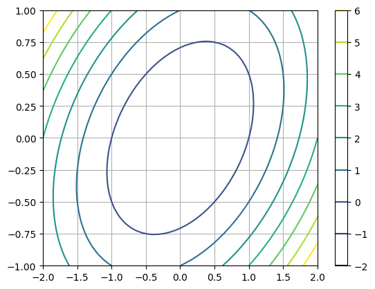
For example, let’s create the contour plot of the function \(z = x^2 - xy + 2y^2 - 1\) over the intervals \(-2 \leq x \leq 2\) and \(-1 \leq y \leq 1\).

x = np.linspace(-2,2,51)
y = np.linspace(-1,1,51)
X,Y = np.meshgrid(x,y)
Z = X**2 - X*Y + 2*Y**2 - 1
plt.contour(X,Y,Z,levels=[-2,-1,0,1,2,3,4,5,6])
plt.grid(True), plt.colorbar()
plt.show()

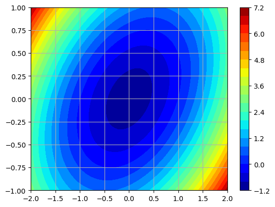
There are several other options:

• Plot a filled contour plot with plt.contourf

• Choose a different colormap with cmap (see Matplotlib colormaps)

• Set the number of levels (as opposed to setting the \(z\) value of each level)

x = np.linspace(-2,2,51)
y = np.linspace(-1,1,51)
X,Y = np.meshgrid(x,y)
Z = X**2 - X*Y + 2*Y**2 - 1
plt.contourf(X,Y,Z,levels=20,cmap='jet')
plt.grid(True), plt.colorbar()
plt.show()

What is meshgrid?

The function np.meshgrid takes vectors

\[ \mathbf{x} = \begin{bmatrix} x_0 & x_1 & \cdots & x_m \end{bmatrix} \hspace{20mm} \mathbf{y} = \begin{bmatrix} y_0 & y_1 & \cdots & y_n \end{bmatrix} \]

and creates the matrices

\[\begin{split} X = \begin{bmatrix} x_0 & x_1 & \cdots & x_m \\ x_0 & x_1 & \cdots & x_m \\ \vdots & \vdots & \ddots & \vdots \\ x_0 & x_1 & \cdots & x_m \end{bmatrix} \hspace{20mm} Y = \begin{bmatrix} y_0 & y_0 & \cdots & y_0 \\ y_1 & y_1 & \cdots & y_1 \\ \vdots & \vdots & \ddots & \vdots \\ y_n & y_n & \cdots & y_n \end{bmatrix} \end{split}\]

Note that the rows of the matrix \(X\) are all equal to the vector \(\mathbf{x}\), and the columns of the matrix \(Y\) are all equal to the vector \(\mathbf{y}\). For example:

x = np.array([-2,-1,0,1,2])
y = np.array([0,0.5,1])

X,Y = np.meshgrid(x,y)

print(X)

[[-2 -1  0  1  2]
 [-2 -1  0  1  2]
 [-2 -1  0  1  2]]

print(Y)

[[0.  0.  0.  0.  0. ]
 [0.5 0.5 0.5 0.5 0.5]
 [1.  1.  1.  1.  1. ]]

What’s the point?!! Think about how we plot a function \(z = f(x,y)\):

1. Choose a vector of \(x\) values.

2. Choose a vector of \(y\) values.

3. Create the grid of points \((x_i,y_j)\).

4. Compute the values \(z_{ji} = f(x_i,y_j)\) at the grid points.

5. Connect adjacent points to create the surface!

The grid of points in the \(xy\)-plane is represented by the “matrix” of points:

\[\begin{split} \begin{bmatrix} (x_0,y_0) & (x_1,y_0) & \cdots & (x_m,y_0) \\ (x_0,y_1) & (x_1,y_1) & \cdots & (x_m,y_1) \\ \vdots & \vdots & \ddots & \vdots \\ (x_0,y_n) & (x_1,y_n) & \cdots & (x_m,y_n) \\ \end{bmatrix} \end{split}\]

Lets write out the matrix of \(z\) values:

\[\begin{split} Z = \begin{bmatrix} z_{0,0} & z_{0,1} & \cdots & z_{0,m} \\ z_{1,0} & z_{1,1} & \cdots & z_{1,m} \\ \vdots & \vdots & \ddots & \vdots \\ z_{n,0} & z_{n,1} & \cdots & z_{n,m} \end{bmatrix} = \begin{bmatrix} f(x_0,y_0) & f(x_1,y_0) & \cdots & f(x_m,y_0) \\ f(x_0,y_1) & f(x_1,y_1) & \cdots & f(x_m,y_1) \\ \vdots & \vdots & \ddots & \vdots \\ f(x_0,y_n) & f(x_1,y_n) & \cdots & f(x_m,y_n) \\ \end{bmatrix} = f(X,Y) \end{split}\]

Note the order of \(i\) and \(j\) in the notation: \(z_{j,i} = f(x_i,y_j)\). Therefore the matrix \(Z\) of \(z\) values is the result of applying the vectorized function \(f(x,y)\) to the matrices \(X\) and \(Y\).

In the end, all we need to do is copy/paste/modify the code above for new examples!

Examples

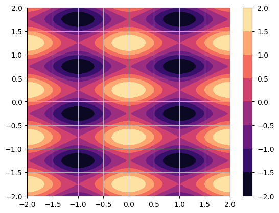
Plot the function \(z = \cos(\pi x) + \sin(2 \pi y)\) over the intervals \(-2 \leq x \leq 2\) and \(-2 \leq y \leq 2\).

x = np.linspace(-2,2,101)
y = np.linspace(-2,2,101)
X,Y = np.meshgrid(x,y)
Z = np.cos(np.pi*X) + np.sin(2*np.pi*Y)
plt.contourf(X,Y,Z,cmap='magma')
plt.grid(True), plt.colorbar()
plt.show()

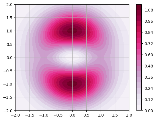
Plot the function \(z = (x^2 + 3y^2)e^{-x^2-y^2}\) over the intervals \(-2 \leq x \leq 2\) and \(-2 \leq y \leq 2\).

x = np.linspace(-2,2,101)
y = np.linspace(-2,2,101)
X,Y = np.meshgrid(x,y)
Z = (X**2 + 3*Y**2)*np.exp(-X**2-Y**2)
plt.contourf(X,Y,Z,levels=20,cmap='PuRd')
plt.grid(True), plt.colorbar()
plt.show()