Vectorization and Plotting

import numpy as np

Vectorization is a fundamental concept in mathematical computing. The idea is simple but very powerful: take any function/operation \(f(x)\) and apply it to a vector \(\mathbf{x} = \begin{bmatrix} x_0 & x_1 & \cdots & x_N \end{bmatrix}\) elementwise simultaneously:

\[ f(\mathbf{x}) = \begin{bmatrix} f(x_0) & f(x_1) & \cdots & f(x_N) \end{bmatrix} \]

The point is that vectorization simplifies our code and our computational thinking and we use it whenever we plot a function with NumPy and Matplotlib.

Basic Plotting Procedure

To plot the graph of a function \(y = f(x)\) over an interval \([a,b]\):

• Choose a finite set of increasing values \(x_0 < x_1 < \cdots < x_N\) with \(x_0 = a\) and \(x_N = b\)

• Compute the corresponding \(y\) values \(f(x_0),f(x_1),\dots,f(x_N)\)

• Connect each pair of consecutive points by a straight line

Let’s make a few simple observations. A larger number \(N\) of \(x\) values over the interval \([a,b]\):

• produces a smoother plot

• requires more computations to generate \(y\) values

• requires more memory to store the \(x\) and \(y\) values

We need to use our own judgement to choose \(N\) large enough so that the plot is smooth but small enough so that the amount of computation and memory required is not too big.

Matplotlib

Matplotlib is the main plotting package in Python. It is a large package with lots of subpackages and we primarily use the subpackages matplotlib.pyplot for 2D plotting. Import using the keyword import and use the alias plt.

import matplotlib.pyplot as plt

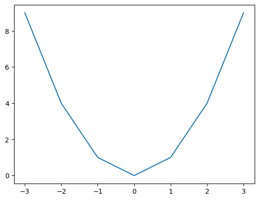
The command plt.plot(x,y) creates the line plot which connects the points defined by the vectors x and y. For example, the following script plots the graph of \(y = x^2\) using 7 points:

x = np.array([-3.,-2.,-1.,0.,1.,2.,3.])
y = np.array([9.,4.,1.,0.,1.,4.,9.])
plt.plot(x,y)
plt.show()

We need more points to plot the function smoothly but it is inefficient to manually enter the values in the vectors x and y as we did above. Plotting is an instance where vectorization is very useful:

• Use the function np.linspace to create a large number of \(x\) values

• Use vector operations and functions to create the corresponding vector of \(y\) values

• Plot with plt.plot(x,y) and add style such as title, colors, line styles, legend, etc.

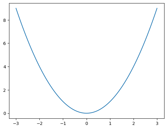
For example, let’s use vectorization to plot \(y = x^2\) on the interval \([-3,3]\) using 100 points:

x = np.linspace(-3,3,100);
y = x**2;
plt.plot(x,y)
plt.show()

Let’s take a closer look at the function np.linspace and vector operation x**2.

See also

Check out Mathematical Pyton > Matplotlib for more about plotting with Matplotlib.

np.linspace

The function np.linspace(a,b,N) creates a vector of values from a to b using N equally spaced points. For example, create a vector of 9 evenly spaced values from 0 to 1:

x = np.linspace(0,1,9)
print(x)

[0.    0.125 0.25  0.375 0.5   0.625 0.75  0.875 1.   ]

The connection between the step size h and the number of points N is given by

\[ h = \frac{b - a}{N - 1} \]

For example, the following commands create a vector x of values from 0 to 1 by step 0.25:

a = 0; b = 1; N = 5; h = (b - a)/(N - 1);
x = np.linspace(a,b,N)

print(h)

0.25

print(x)

[0.   0.25 0.5  0.75 1.  ]

Vectorized Functions

All the mathematical functions in NumPy such as np.sin, np.cos and np.exp are vectorized. This means that we can apply a function to a vector and the result is the vector of function values. In other words, if \(f(x)\) is a vectorized function and \(\mathbf{x} = \begin{bmatrix} x_0 & x_1 & \cdots & x_N \end{bmatrix}\) is a vector then

\[ f(\mathbf{x}) = \begin{bmatrix} f(x_0) & f(x_1) & \cdots & f(x_N) \end{bmatrix} \]

For example, the vectors y1 and y2 computed below are identical:

y1 = np.array([np.sin(0),np.sin(np.pi/4),np.sin(np.pi/2),np.sin(3*np.pi/4),np.sin(np.pi)])
print(y1)

[0.00000000e+00 7.07106781e-01 1.00000000e+00 7.07106781e-01
 1.22464680e-16]

x = np.array([0,np.pi/4,np.pi/2,3*np.pi/4,np.pi])
y2 = np.sin(x)
print(y2)

[0.00000000e+00 7.07106781e-01 1.00000000e+00 7.07106781e-01
 1.22464680e-16]

Note that 1e-16 is scientific notation for \(10^{-16}\) which is very, very small. When we do numerical computations, there is sometimes some rounding error. But we usually interpret numbers like 1e-16 as 0.

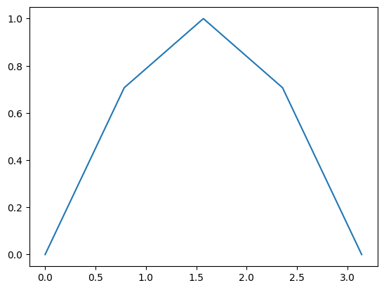
Let’s use just these 5 points to plot \(y = \sin(x)\):

x = np.array([0,np.pi/4,np.pi/2,3*np.pi/4,np.pi])
y = np.sin(x)
plt.plot(x,y)
plt.show()

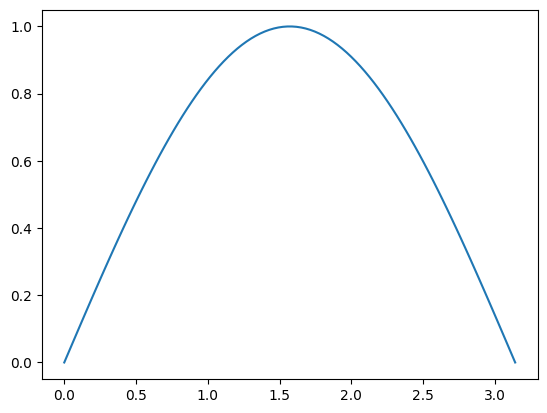
Clearly we need more points to plot the function smoothly. Let’s use np.linspace to plot the function \(y = \sin(x)\) over the interval \([0,\pi]\) using 100 points:

x = np.linspace(0,np.pi,100)
y = np.sin(x)
plt.plot(x,y)
plt.show()

Vectorized Arithmetic Operations

Vector addition is defined by adding vectors entry-by-entry

\[\begin{split} \mathbf{x} + \mathbf{y} = \begin{bmatrix} x_0 \\ x_1 \\ \vdots \\ x_N \end{bmatrix} + \begin{bmatrix} y_0 \\ y_1 \\ \vdots \\ y_N \end{bmatrix} = \begin{bmatrix} x_0 + y_0 \\ x_1 + y_1 \\ \vdots \\ x_N + y_N \end{bmatrix} \end{split}\]

Scalar multiplication is defined by multiplying a vector entry-by-entry by a scalar

\[\begin{split} c \mathbf{x} = c \begin{bmatrix} x_0 \\ x_1 \\ \vdots \\ x_N \end{bmatrix} = \begin{bmatrix} c x_0 \\ c x_1 \\ \vdots \\ c x_N \end{bmatrix} \end{split}\]

Then how could we define \(\mathbf{x} + c\) where \(\mathbf{x}\) is a vector and \(c\) is a scalar? Perform the operation entry-by-entry

\[\begin{split} \mathbf{x} + c = \begin{bmatrix} x_0 \\ x_1 \\ \vdots \\ x_N \end{bmatrix} + c = \begin{bmatrix} x_0 + c \\ x_1 + c \\ \vdots \\ x_N + c \end{bmatrix} \end{split}\]

We also define vectorized multiplication, division and exponentiation:

Vectorized Operation	NumPy Syntax
addition	+
subtraction	-
multiplication	*
division	/
exponentiation	**

For example, the following script creates identical vectors y1 and y2:

y1 = np.array([(-3.)**2,(-2.)**2,(-1.)**2,0.**2,1.**2,2.**2,3.**2])
print(y1)

[9. 4. 1. 0. 1. 4. 9.]

x = np.array([-3.,-2.,-1.,0.,1.,2.,3.])
y2 = x**2
print(y2)

[9. 4. 1. 0. 1. 4. 9.]

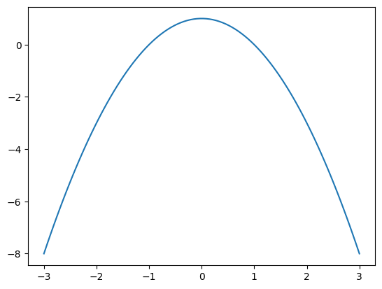
Use vectorization to plot \(f(x) = 1 - x^2\) over the interval \([-3,3]\):

x = np.linspace(-3,3,100);
y = 1 - x**2;
plt.plot(x,y)
plt.show()

Create the vector of values \(y = xe^{-x}\) for \(x\) from 0 to 1 with step 0.25:

x = np.linspace(0,1,5)
y = x*np.exp(-x)
print(y)

[0.         0.1947002  0.30326533 0.35427491 0.36787944]

The values \(y_k\) in the vector \(\mathbf{y}\) correspond to \(x_k\) in the vector \(\mathbf{x}\) by:

\[ y_k = x_k e^{-x_k} \]

The simple code above produces the same vector as the more verbose code below:

y = np.array([0*np.exp(-0),0.25*np.exp(-0.25),0.5*np.exp(-0.5),0.75*np.exp(-0.75),np.exp(-1)])
print(y)

[0.         0.1947002  0.30326533 0.35427491 0.36787944]

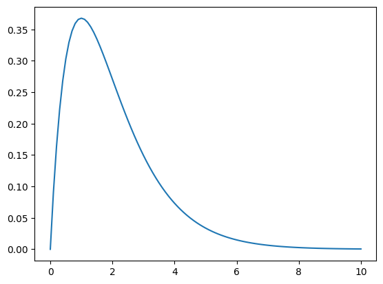
Use vectorization to plot \(f(x) = x e^{-x}\) over the interval \([0,10]\):

x = np.linspace(0,10,101)
y = x*np.exp(-x)
plt.plot(x,y)
plt.show()

More Plotting Examples

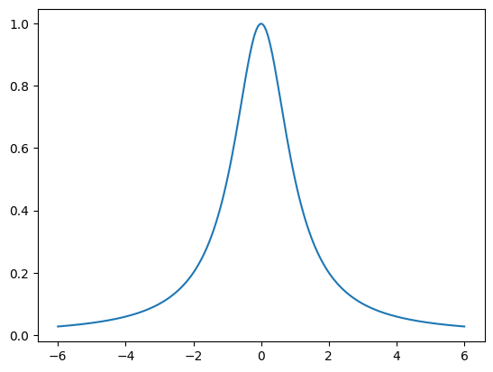
Plot \(f(x) = \displaystyle \frac{1}{1 + x^2}\) over the interval \([-6,6]\):

x = np.linspace(-6,6,200)
y = 1/(1 + x**2)
plt.plot(x,y)
plt.show()

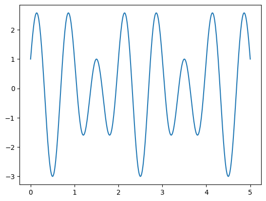
Plot \(f(x) = \cos(2 \pi x) + 2 \sin(3 \pi x)\) over the interval \([0,5]\):

x = np.linspace(0,5,500);
y = np.cos(2*np.pi*x) + 2*np.sin(3*np.pi*x);
plt.plot(x,y)
plt.show()

Exercises

Exercise 1. Without running the code, predict the values y[0], y[10] and y[20] in the code below.

x = np.linspace(-1,1,21)
y = 1 + x + x**2

Exercise 2. Without running the code, predict the values y[0], y[50] and y[100] in the code below.

x = np.linspace(0,2,101);
y = x*exp(-x**2);

Exercise 3. Plot \(f(x) = \ln(1 + x)\) over the interval \([0,10]\).

Exercise 4. Plot \(f(x) = \arctan(x)\) over the interval \([-5,5]\).

Exercise 5. Plot \(f(x) = 1/\sqrt{1 + x^2}\) over the interval \([4,4]\).

Exercise 6. Plot \(f(x) = e^{\sin(x)}\) over the interval \([0,4\pi]\).