Euler’s Method

Most differential equations cannot be solved analytically in terms of elementary functions. So what do we do? We can always approximate. Euler’s method is the simplest numerical method for approximating solutions of differential equations.

import numpy as np
import matplotlib.pyplot as plt

Derivation

Consider a first order differential equation with an initial condition:

\[ y' = f(t,y) \ , \ \ y(t_0)=y_0 \]

The idea behind Euler’s method is:

1. Contruct the equation of the tangent line to the unknown function \(y(t)\) at \(t=t_0\):

   \[ y = y(t_0) + f(t_0,y_0)(t - t_0) \]

   where \(y'(t_0) = f(t_0,y_0)\) is the slope of \(y(t)\) at \(t=t_0\).

2. Use the tangent line to approximate \(y(t)\) at a small time step \(t_1 = t_0 + h\):

   \[ y_1 = y_0 + f(t_0,y_0)(t_1 - t_0) \]

   where \(y_1 \approx y(t_1)\).

3. Repeat! Construct the line at \((t_n,y_n)\) of slope \(f(t_n,y_n)\) and compute \(y_{n+1}\) at \(t_{n+1} = t_n + h\).

The formula for Euler’s method defines a recursive sequence:

\[ y_{n+1} = y_n + f(t_n,y_n)(t_{n+1} - t_n) \ , \ \ y_0 = y(t_0) \]

where \(y_n \approx y(t_n)\) for each \(n\). If we choose equally spaced \(t\) values then the formula becomes:

\[ y_{n+1} = y_n + f(t_n,y_n)h \ \ , \ \ y_0 = y(t_0) \ , \ \ t_n = t_0 + nh \]

with time step \(h = t_{n+1} - t_n\). If we implement \(N\) iterations of Euler’s method from \(t_0\) to \(t_f\) then the time step is

\[ h = \frac{t_f - t_0}{N} \]

Note two very important points about Euler’s method and numerical methods in general:

• A smaller time step \(h\) reduces the error in the approximation.

• A smaller time step \(h\) requires more computations!

Implementation

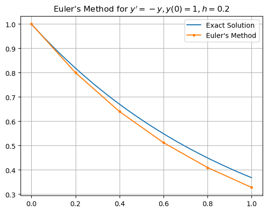
Let’s apply Euler’s method to the equation \(y' = -y, y(0)=1\). We can solve the equation analytically to find \(y(t) = e^{-t}\) and so we can compare the approximation to the exact solution.

The Python code below accomplishes the following tasks:

1. Define the right hand side of the equation \(y' = f(t,y)\) as a Python function f(t,y).

2. Define the initial value \(t_0\) and final value \(t_f\) and the number \(N\) of iterations to compute.

3. Create a vector t of \(N+1\) equally spaced values from \(t_0\) to \(t_f\)

4. Define the initial value \(y_0 = y(t_0)\), initialize a vector y of zeros of the same length as the vector t.

5. Initialize the first entry y[0] of vector y as the initial value \(y_0\).

6. Compute each value \(y_{n+1} = y_n + f(t_n,y_n) h\) for \(n=0,\dots,N-1\) and update the entry y[n+1].

f = lambda t,y: -y

t0 = 0; tf = 1; N = 5; h = (tf - t0)/N;
t = np.linspace(t0,tf,N+1)

y0 = 1
y = np.zeros(len(t))
y[0] = y0

for n in range(N):
    y[n+1] = y[n] + f(t[n],y[n])*h

Print the vector t to see that the first entry is \(t_0\), the last value is \(t_f\), all values are equally spaced by step size \(h\) and that there are \(N+1\) entries.

t

array([0. , 0.2, 0.4, 0.6, 0.8, 1. ])

Print the vector y to see that the first entry is \(y_0\) and that there are \(N+1\) entries.

y

array([1.     , 0.8    , 0.64   , 0.512  , 0.4096 , 0.32768])

We know the exact solution is \(y(t) = e^{-t}\). Let’s plot the exact solution with the approximation.

t_exact = np.linspace(0,1,100)
y_exact = np.exp(-t_exact)
plt.plot(t_exact,y_exact,label='Exact Solution')
plt.plot(t,y,'.-',label="Euler's Method")
plt.grid(True), plt.legend(), plt.title("Euler's Method for $y' = -y, y(0) = 1, h = 0.2$")
plt.show()

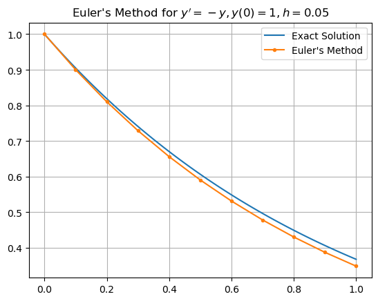
Increasing the number \(N\) of iterations gives a better approximation.

f = lambda t,y: -y

t0 = 0; tf = 1; N = 10; h = (tf - t0)/N;
t = np.linspace(t0,tf,N+1)

y0 = 1
y = np.zeros(len(t))
y[0] = y0

for n in range(N):
    y[n+1] = y[n] + f(t[n],y[n])*h

t_exact = np.linspace(0,1,100)
y_exact = np.exp(-t_exact)

plt.plot(t_exact,y_exact,label='Exact Solution')
plt.plot(t,y,'.-',label="Euler's Method")
plt.grid(True), plt.legend(), plt.title("Euler's Method for $y' = -y, y(0) = 1, h = 0.05$")
plt.show()

Example

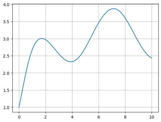
Consider the equation \(y' = \cos(t) + \sin(y), y(0)=1\). This is a nonlinear, nonseparable equation and there is no method to solve it analytically using elementary functions. Let’s approximate the solution using Euler’s method.

f = lambda t,y: np.cos(t) + np.sin(y)

t0 = 0; tf = 10; N = 500; h = (tf - t0)/N;
t = np.linspace(t0,tf,N+1)

y0 = 1
y = np.zeros(len(t))
y[0] = y0

for n in range(N):
    y[n+1] = y[n] + f(t[n],y[n])*h

plt.plot(t,y)
plt.grid(True)
plt.show()

Euler’s Method Function

Let’s define a function called odeEuler to implement Euler’s method. The function takes input parameters f, t and y0 and returns y where:

• f is a function which represents the right hand side of a first order differential equation \(y'=f(t,y)\)

• t is a vector of \(t\) values

• y0 is the initial value \(y_0 = y(t_0)\) where \(t_0\) is the first entry t[0] of the vector t

def odeEuler(f,t,y0):
    y = np.zeros(len(t))
    y[0] = y0
    for n in range(len(t)-1):
        y[n+1] = y[n] + f(t[n],y[n])*(t[n+1] - t[n])
    return y

Let’s use the function on the same example as above.

f = lambda t,y: np.cos(t) + np.sin(y)
t0 = 0; tf = 10; N = 1000;
t = np.linspace(t0,tf,N+1)
y0 = 1
y = odeEuler(f,t,y0)
plt.plot(t,y,'C0')
plt.grid(True)
plt.show()

Now let’s use the function in a for loop to plot solutions of the example above for many initial conditions.

f = lambda t,y: np.cos(t) + np.sin(y)
t0 = 0; tf = 10; N = 500;
t = np.linspace(t0,tf,N+1)

for y0 in range(-3,10):
    y = odeEuler(f,t,y0)
    plt.plot(t,y,'C0')

plt.grid(True)
plt.show()

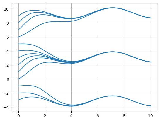
It seems that solutions converge to oscillating functions at different height depending on the initial condition.