Slope Fields

Most differential equations cannot be solved analytically in terms of elementary functions. So what do we do? We can always approximate! A slope field is a visualization of the slopes of solutions of a first order differential equation. We can study the slope field of an equation to approximate quantitative properties and describe qualitative properties of solutions.

import numpy as np
import matplotlib.pyplot as plt

What is a Slope Field?

Let \(y' = f(t,y)\) be a first order differential equation. The function \(f(t,y)\) gives us complete information about the slope of any solution of the equation. In particular, the number \(f(t,y)\) at point \((t,y)\) is the slope at \(t\) of the unique solution \(y(t)\) which passes through the point \((t,y)\). Therefore if we plot a short line of slope \(f(t,y)\) at a bunch of points in the \(ty\)-plane then the resulting figure should show roughly what solutions look like.

Consider a first order differential equation \(y' = f(t,y)\). We can represent the function \(f(t,y)\) as a Python function. For example, consider the equation \(y' = -ty\). The code below defines a Python function f.

f = lambda t,y: -t*y

The keyword lambda starts the function definition. The symbols t,y set the input variables as t and y, the colon : begins the function formula -t*y where * is multiplication. Plug in some values for t and y to verify. For example, \(f(1.2,-0.2) = -(1.2)(-0.2) = 0.24\).

f(1.2,-0.2)

0.24

Now the goal is to use the Python function f to compute slopes at a grid of points in the \(ty\)-plane and plot the slope field.

slopefield

Define a function called slopefield which takes input parameters f, tinterval, yinterval, tstep and ystep where:

• f is a Python function which represents the right hand side of a first order differential equation \(y' = f(t,y)\)

• tinterval is a Python list of length 2 which represents the interval \([t_0,t_1]\) of the grid in the slope field

• yinterval is a Python list of length 2 which represents the interval \([y_0,y_1]\) of the grid in the slope field

• tstep is the step size between points in the \(t\) direction

• ystep is the step size between points in the \(y\) direction

The function accomplishes the following tasks:

• Create the vector t of values from \(t_0\) to \(t_1\) with step size tstep

• Create the vector y of values from \(y_0\) to \(y_1\) with step size ystep

• Define a length \(L\) for the lines in the slope field (small enough not to overlap)

• For each \(t_i\) and \(y_j\) in the grid, compute \(m_{ij} = f(t_i,y_j)\) and plot a line of slope \(m_{ij}\) and length \(L\)

def slopefield(f,tinterval,yinterval,tstep,ystep):
    t = np.arange(tinterval[0],tinterval[1],tstep)
    y = np.arange(yinterval[0],yinterval[1],ystep)
    L = 0.7*min(tstep,ystep)
    for i in range(len(t)):
        for j in range(len(y)):
            slope = f(t[i],y[j])
            theta = np.arctan(slope)
            dy = L*np.sin(theta)
            dt = L*np.cos(theta)
            plt.plot([t[i],t[i] + dt],[y[j],y[j] + dy],'b')

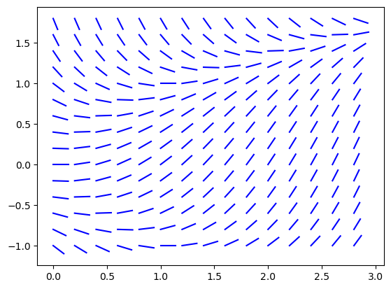
For example, let’s plot the slope field for the equaiton \(y' = t - y^2\) over the intervals \(0 \leq t \leq 3\) and \(-1 \leq y \leq 2\) with step size 0.2 in both directions.

f = lambda t,y: t - y**2
slopefield(f,[0,3],[-1,2],0.2,0.2)

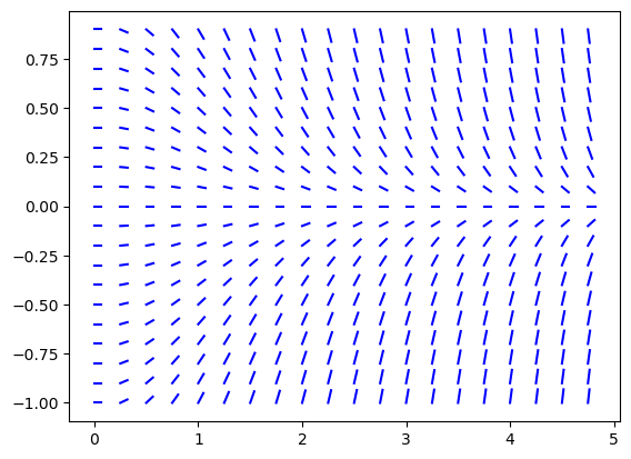
Now let’s plot the slope field of \(y' = -ty\) over the intervals intervals \(0 \leq t \leq 5\) and \(-1 \leq y \leq 1\) with step size 0.25 in the \(t\) direction and step size 0.1 in the \(y\) direction.

f = lambda t,y: -t*y
slopefield(f,[0,5],[-1,1],0.25,0.1)

Examples

Autonomous Equation

Plot the slope field of \(y' = 1 - y^2\).

f = lambda t,y: 1 - y**2
slopefield(f,[0,4],[-2,2],0.2,0.2)

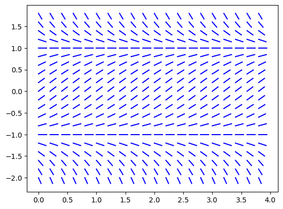
The equation is autonomous since the right hand function \(f(t,y) = 1-y^2\) does not depend on \(t\). We can also see this in the slope field: the slopes are constant in the \(t\) direction. The slope field also shows that \(y = 1\) is a stable equilibirum solution and \(y=-1\) is an unstable equilibrium solution.

Convergent Solutions

Plot the slope field of \(\displaystyle y' = -\frac{y}{2 + \cos(t)}\).

f = lambda t,y: -y/(2 + np.cos(t))
slopefield(f,[0,10],[-5,5],0.5,0.5)

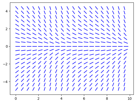
The figure suggests that \(y(t) \to 0\) as \(t \to \infty\) for any solution but we need some more analysis to prove this.