Slope Fields

Most differential equations cannot be solved analytically in terms of elementary functions. So what do we do? We can always approximate. A slope field is a visualization of the slopes of solutions of a first order differential equation. We can study the slope field of an equation to approximate quantitative properties and describe qualitative properties of solutions.

import numpy as np
import matplotlib.pyplot as plt

What is a Slope Field?

Let \(y' = f(t,y)\) be a first order differential equation. The function \(f(t,y)\) gives us complete information about the slope of any solution of the equation. In particular, the number \(f(t,y)\) at point \((t,y)\) is the slope at \(t\) of the unique solution \(y(t)\) which passes through the point \((t,y)\). Therefore if we plot a short line of slope \(f(t,y)\) at a bunch of points in the \(ty\)-plane then the resulting figure should show roughly what solutions look like.

Implementation

To create a slope field, we define a grid of points in the \(ty\)-plane, compute the slope \(m_{ij} = f(t_i,y_j)\) at each point \((t_i,y_j)\) in the grid, and then plot a line of slope \(m_{ij}\) at each point. The Python code below accomplishes the following tasks:

1. Define the right had side of the differential equation \(y' = f(t,y)\) as a Python function.

2. Choose an interval \([t_0,t_f]\) and the number \(N\) of points in the grid from \(t_0\) to \(t_f\).

3. Create the vector (of length \(N\)) of \(t\) values from \(t_0\) to \(t_f\).

4. Choose an interval \([y_0,y_f]\) and the number \(M\) of points in the grid from \(y_0\) to \(y_f\).

5. Create the vector (of length \(M\)) of \(y\) values from \(y_0\) to \(y_f\).

6. Define a length \(L\) for the lines in the slope field (small enough so that the lines are clear and don’t overlap).

7. For each \(t_i\) and \(y_j\) in the grid, compute \(m_{ij} = f(t_i,y_j)\) and plot a line of slope \(m_{ij}\) and length \(L\).

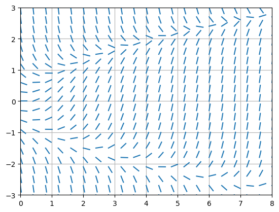
Let’s plot the slope field for the equaiton \(y' = t - y^2\) for \(0 \leq t \leq 3\) and \(-1 \leq y \leq 2\).

f = lambda t,y: t - y**2

t0 = 0; tf = 8; N = 21;
t = np.linspace(t0,tf,N)

y0 = -3; yf = 3; M = 21;
y = np.linspace(y0,yf,M)

L = 0.7*min((tf-t0)/(N-1),(yf-y0)/(M-1));

for i in range(N):
    for j in range(M):
        m = f(t[i],y[j])
        theta = np.arctan(m)
        dy = L*np.sin(theta)
        dt = L*np.cos(theta)
        plt.plot([t[i],t[i] + dt],[y[j],y[j] + dy],'C0')

plt.grid(True), plt.axis([t0,tf,y0,yf])
plt.show()

How do we know how to choose parameters \(t_0,t_f,y_0,y_f,N,M,L\)? Let’s make some observations:

• Choose different intervals \([t_0,t_f]\) and \([y_0,y_f]\) to focus on different parts of the \(ty\)-plane.

• Choose larger values \(N\) and \(M\) to make a finer grid (but not too large such that the plot is unclear).

For example, there seems to be some interesting behaviour of solutions of the equation \(y' = t - y^2\) near \(t=0\) and \(y=-0.75\). Let’s focus our slope field near that point:

f = lambda t,y: t - y**2

t0 = 0; tf = 1; N = 21;
t = np.linspace(t0,tf,N)

y0 = -1.25; yf = -0.25; M = 21;
y = np.linspace(y0,yf,M)

L = 0.7*min((tf-t0)/(N-1),(yf-y0)/(M-1));

for i in range(N):
    for j in range(M):
        m = f(t[i],y[j])
        theta = np.arctan(m)
        dy = L*np.sin(theta)
        dt = L*np.cos(theta)
        plt.plot([t[i],t[i] + dt],[y[j],y[j] + dy],'C0')

plt.grid(True), plt.axis([t0,tf,y0,yf])
plt.show()

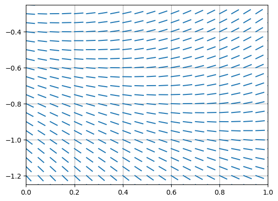
We may conclude from inspecting the plot that there exists an initial value \(\alpha\) between \(-0.7\) and \(-0.8\) such that if \(y(t)\) is a solution which satisfies \(y(0) < \alpha\) then \(\lim_{t \to \infty} y(t) = -\infty\).

Examples

Autonomous Equation

Plot the slope field of \(y' = 1 - y^2\). Copy, paste and modify the code above into the cell below:

f = lambda t,y: 1 - y**2

t0 = 0; tf = 4; N = 21;
t = np.linspace(t0,tf,N)

y0 = -2; yf = 2; M = 21;
y = np.linspace(y0,yf,M)

L = 0.7*min((tf-t0)/(N-1),(yf-y0)/(M-1));

for i in range(N):
    for j in range(M):
        m = f(t[i],y[j])
        theta = np.arctan(m)
        dy = L*np.sin(theta)
        dt = L*np.cos(theta)
        plt.plot([t[i],t[i] + dt],[y[j],y[j] + dy],'C0')

plt.grid(True), plt.axis([t0,tf,y0,yf])
plt.show()

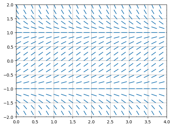
The equation is autonomous since the right hand function \(f(t,y) = 1-y^2\) does not depend on \(t\). We can also see this in the slope field: the slopes are constant in the \(t\) direction. The slope field also shows that \(y = 1\) is a stable equilibirum solution and \(y=-1\) is an unstable equilibrium solution.

Convergent Solutions

Plot the slope field of \(\displaystyle y' = -\frac{y}{2 + \cos(t)}\). Copy, paste and modify the code above into the cell below:

f = lambda t,y: -y/(2 + np.cos(t))

t0 = 0; tf = 10; N = 31;
t = np.linspace(t0,tf,N)

y0 = -5; yf = 5; M = 31;
y = np.linspace(y0,yf,M)

L = 0.7*min((tf-t0)/(N-1),(yf-y0)/(M-1));

for i in range(N):
    for j in range(M):
        m = f(t[i],y[j])
        theta = np.arctan(m)
        dy = L*np.sin(theta)
        dt = L*np.cos(theta)
        plt.plot([t[i],t[i] + dt],[y[j],y[j] + dy],'C0')

plt.grid(True), plt.axis([t0,tf,y0,yf])
plt.show()

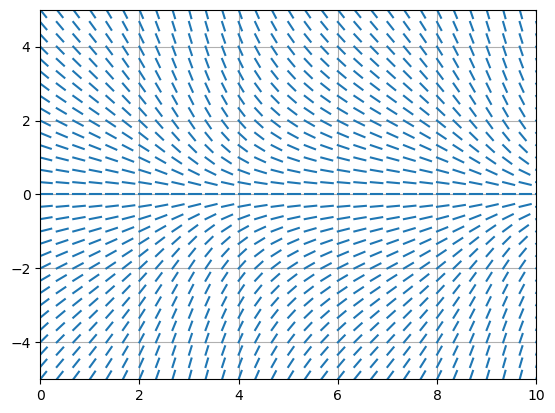
We may conclude from the slope field that if \(y(t)\) is any solution such that \(|y(0)|\leq 5\) then \(y(t) \to 0\) as \(t \to \infty\). The figure suggests that \(y(t) \to 0\) as \(t \to \infty\) for any solution but we need some more analysis to prove this.