Probability Distributions

import numpy as np
import matplotlib.pyplot as plt

Random Variables

Consider an experiment or a random event such as flipping a coin or measuring wind speed and direction at a specific time and location. A random variable is a function that associates a numerical value with the outcome of an experiment or random event. If the range of values of a random variable \(X\) is finite or countable (like the set of integers) then we call \(X\) a discrete random variable. If the range of values of a random variable \(X\) is uncountably infinite (like the set of real numbers \(\mathbb{R}\)) then we call \(X\) a continuous random variable. For example:

• Flip a coin and let \(X = 1\) if the outcome is heads and \(X = 0\) if the outcome is tails. Then \(X\) is a discrete random variable.

• Let \(X\) be the total number of points scored in a basketball game. Then \(X\) is a positive integer and so \(X\) is a discrete random variable.

• Let \(X\) be the temperature measured at a specific time and location. The possible values of \(X\) is the set of positive real numbers and so \(X\) is a continous random variable.

• Throw a dart at a dartboard and let \(X\) be the distance from where the dart lands to the center of the baord. The possible values of \(X\) is again the set of positive real numbers so \(X\) is a continuous random variable.

• Let \(X\) be the wind direction measured at a specific time and location. The possible values of \(X\) is the set \([0,2 \pi]\) and so \(X\) is a continous random variable.

Probability Density Functions

A probability density function is a function \(f : \mathbb{R} \rightarrow \mathbb{R}\) such that \(f(x) \ge 0\) for all \(x \in \mathbb{R}\) and

\[ \int_{-\infty}^{\infty} f(x) \, dx \]

A probability density function determines a continuous random variable. In other words, the probability distribution of a continuous random variable \(X\) is given by the density function \(f_X(x)\) if

\[ P(a \le X \le b) = \int_a^b f(x) \, dx \]

Mean and Variance

Let \(X\) be a continuous random variable with probability density function \(f_X(x)\). The mean of \(X\) is

\[ \mu = \int_{-\infty}^{\infty} x f_X(x) \, dx \]

The mean describes the central value in the distribution of \(X\). The variance of \(X\) is

\[ \sigma^2 = \int_{-\infty}^{\infty} (x - \mu)^2 f_X(x) \, dx \]

The variance is the average value of the squared distance from the mean \((x - \mu)^2\). The variance describes how spread out the distribution of \(X\) is.

Scaling and Shifting

If \(f(x)\) is a probability density function then the shifted function \(f(x - b)\) is also a density function for any \(b \in \mathbb{R}\). Let’s see why this is true. First, \(f(x - b) \geq 0\) for all \(x \in \mathbb{R}\) since \(f(x) \geq 0\) for all \(x\). Second, compute the integral using the substitution \(y = x- b\), \(dy = dx\)

\[ \int_{-\infty}^{\infty} f(x - b) \, dx = \int_{-\infty}^{\infty} f(y) \, dy = 1 \]

Similarly, if \(f(x)\) is a density function then the scaled function \(a f(ax)\) is also a density function for any \(a > 0\). Let’s see why this is true. First, \(a f(a x) \geq 0\) for all \(x \in \mathbb{R}\) since \(f(x) \geq 0\) for all \(x\) and \(a > 0\). Second, compute the integral using the substitution \(y = ax\), \(dy = a dx\)

\[ \int_{-\infty}^{\infty} af(ax) \, dx = \int_{-\infty}^{\infty} f(y) \, dy = 1 \]

Normal Distribution

The standard normal distribution is given by the probability density function

\[ f(x) = \frac{1}{\sqrt{2 \pi}} e^{-x^2/2} \]

The coefficient \(\frac{1}{\sqrt{2 \pi}}\) comes from the integral formula

\[ \int_0^{\infty} e^{-x^2} dx = \frac{\sqrt{\pi}}{2} \]

See Wikipedia: Error Function. If we scale the function by \(1/\sigma\) and shift by \(\mu\) we get the normal distribution with mean \(\mu\) and variance \(\sigma^2\)

\[ f(x) = \frac{1}{\sigma \sqrt{2 \pi}} e^{-(x - \mu)^2/2\sigma^2} \]

We denote the normal distribution by \(N(\mu,\sigma^2)\).

Let’s plot the normal distrbution for different values of the mean \(\mu\). Increasing the value \(\mu\) simply shifts the curve to the right.

normal = lambda x,mu,sigma: 1/(sigma*np.sqrt(2*np.pi))*np.exp(-(x - mu)**2/(2*sigma**2))
x = np.linspace(-5,10,200)

plt.figure(figsize=(10,4))
for mu in range(0,6):
    y = normal(x,mu,1)
    plt.plot(x,y)
plt.title('Normal Distribution $N(\mu,\sigma^2)$ for $\sigma=1$')
plt.legend(['$\mu=0$','$\mu=1$','$\mu=2$','$\mu=3$','$\mu=4$'])
plt.grid(True)
plt.show()

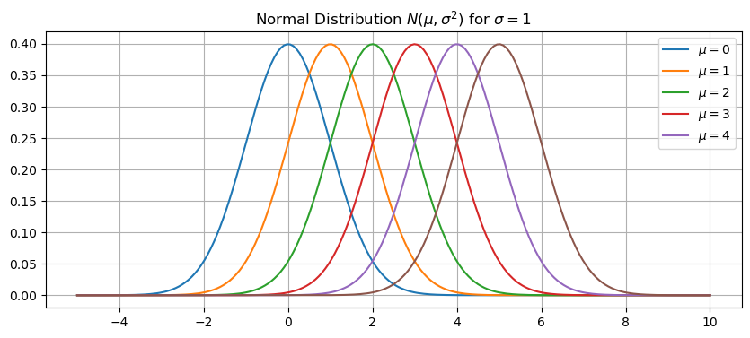
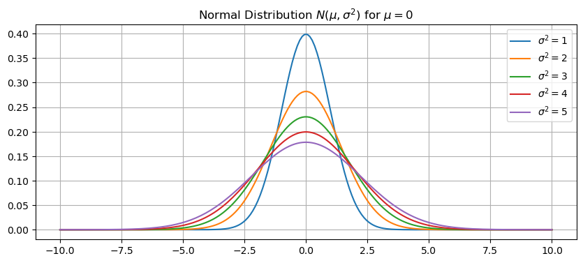
Let’s plot the normal distrbution for different values of the variance \(\sigma^2\). Increasing the value \(\sigma\) flattens and widens the curve.

x = np.linspace(-10,10,200)
plt.figure(figsize=(10,4))
for sigma2 in range(1,6):
    sigma = np.sqrt(sigma2)
    y = normal(x,0,sigma)
    plt.plot(x,y)
plt.title('Normal Distribution $N(\mu,\sigma^2)$ for $\mu=0$')
plt.legend(['$\sigma^2=1$','$\sigma^2=2$','$\sigma^2=3$','$\sigma^2=4$','$\sigma^2=5$'])
plt.grid(True)
plt.show()

See also

Check out Wikipedia: Normal Distribution for more information.

Uniform Distribution

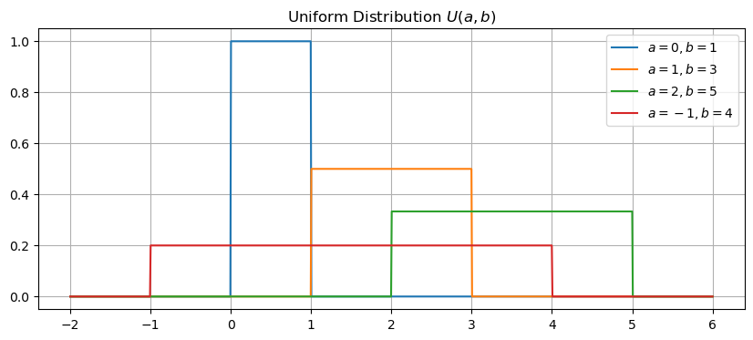
The uniform distribution (with parameters \(a < b\)) is given by the probability density function

\[\begin{split} f(x) = \left\{ \begin{array}{ccc} \frac{1}{b-a} & , & a \le x \le b \\ 0 & , & \text{otherwise} \end{array} \right. \end{split}\]

We denote the uniform distribution by \(U(a,b)\). The mean and variance are given by

\[ \mu = \frac{b+a}{2} \hspace{1in} \sigma^2 = \frac{(b-a)^2}{12} \]

Let’s plot the uniform distrbution for different values of \(a\) and \(b\). Use the function np.heaviside to construct the probability density function (see documentation).

plt.figure(figsize=(10,4))
x = np.linspace(-2,6,1000)
uniform = lambda x,a,b: 1/(b-a)*(np.heaviside(x-a,1) - np.heaviside(x-b,1))
for a,b in [(0,1),(1,3),(2,5),(-1,4)]:
    y = uniform(x,a,b)
    plt.plot(x,y)
plt.title('Uniform Distribution $U(a,b)$')
plt.legend(['$a=0,b=1$','$a=1,b=3$','$a=2,b=5$','$a=-1,b=4$'])
plt.grid(True)
plt.show()

See also

Check out Wikipedia: Uniform Distribution for more information.

Exponential Distribution

The exponential distribution (with parameter \(\lambda\)) is given by the probability density function

\[\begin{split} f(x) = \left\{ \begin{array}{ccc} \lambda e^{- \lambda x} & , & x \ge 0 \\ 0 & , & x < 0 \end{array} \right. \end{split}\]

We denote the exponential distribution by \(Exp(\lambda)\). The mean and variance are given by

\[ \mu = \frac{1}{\lambda} \hspace{1in} \sigma^2 = \frac{1}{\lambda^2} \]

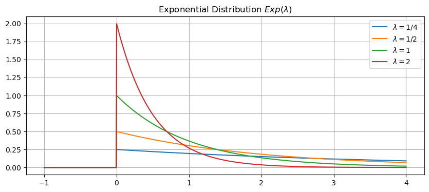
Let’s plot the exponential distrbution for different values of \(\lambda\).

plt.figure(figsize=(10,4))
x = np.linspace(-1,4,1000)
exponential = lambda x,lam: lam*np.exp(-lam*x)*np.heaviside(x,1)
for lam in [.25,.5,1,2]:
    y = exponential(x,lam)
    plt.plot(x,y)
plt.title('Exponential Distribution $Exp(\lambda)$')
plt.legend(['$\lambda=1/4$','$\lambda=1/2$','$\lambda=1$','$\lambda=2$'])
plt.grid(True)
plt.show()

See also

Check out Wikipedia: Exponential Distribution for more information.

Gamma Distribution

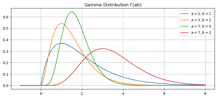
The gamma distribution (with parameters \(\alpha\) and \(\beta\)) is given by the probability density function

\[\begin{split} f(x) = \left\{ \begin{array}{ccc} \displaystyle \frac{\beta^{\alpha}}{\Gamma(\alpha)} x^{\alpha - 1} e^{-\beta x} & , & x \ge 0 \\ 0 & , & x < 0 \end{array} \right. \end{split}\]

where \(\Gamma\) is the Gamma function. We denote the gamma distribution by \(\Gamma(\alpha,\beta)\). Note that \(Exp(\lambda) = \Gamma(1,\lambda)\) The mean and variance are given by

\[ \mu = \frac{\alpha}{\beta} \hspace{1in} \sigma^2 = \frac{\alpha}{\beta^2} \]

Let’s plot the gamma distrbution for different values of \(\alpha\) and \(\beta\). Use the function scipy.special.gamma to compute values of the gamma function \(\Gamma(x)\).

import scipy.special as sps

plt.figure(figsize=(10,4))
x = np.linspace(-1,8,1000)
gamma = lambda x,alpha,beta: beta**alpha/sps.gamma(alpha)*x**(alpha - 1)*np.exp(-beta*x)*np.heaviside(x,1)
for alpha,beta in [(2,1),(3,2),(7,4),(7,2)]:
    y = gamma(x,alpha,beta)
    plt.plot(x,y)
plt.title('Gamma Distribution $\Gamma(a b)$')
plt.legend(['$a=2,b=1$','$a=3,b=2$','$a=7,b=4$','$a=7,b=2$'])
plt.grid(True)
plt.show()