Logistic Function

import numpy as np
import matplotlib.pyplot as plt

Definition and Properties

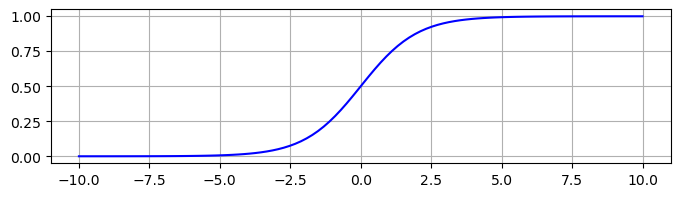
The logistic function is \(\sigma(x) = \displaystyle \frac{1}{1 + e^{-x}}\). Plot the logistic function over the interval \([-10,10]\).

x = np.linspace(-10,10,100)
y = 1/(1 + np.exp(-x))
plt.figure(figsize=(8,2))
plt.plot(x,y,'b'), plt.grid(True)
plt.show()

The \(y\)-intercept is

\[ \sigma(0) = \frac{1}{2} \]

We can see that \(0 < \sigma(x) < 1\) for all \(x\) and the limits at infinity are

\[ \lim_{x \to +\infty} \sigma(x) = 1 \hspace{20mm} \lim_{x \to -\infty} \sigma(x) = 0 \]

Compute the derivative

\[ \sigma'(x) = \frac{e^{-x}}{(1 + e^{-x})^2} \]

The function \(\sigma(x)\) satisfies the differential equation \(\sigma' = \sigma(1 - \sigma)\) since

\[ \sigma(x) \left( 1 - \sigma(x) \right) = \frac{1}{1 + e^{-x}} \left( 1 - \frac{1}{1 + e^{-x}} \right) = \frac{1}{1 + e^{-x}} \left( \frac{e^{-x}}{1 + e^{-x}} \right) = \frac{e^{-x}}{(1 + e^{-x})^2} \]

The slope at the \(y\)-intercept is

\[ \sigma'(0) = \frac{1}{4} \]

The limits at infinity of the derivative are

\[ \lim_{x \to +\infty} \sigma'(x) = 0 \hspace{20mm} \lim_{x \to -\infty} \sigma'(x) = 0 \]

Weight and Bias Parameters

The logistic function with weight \(W\) and bias \(b\) is

\[ \sigma(x; W,b) = \frac{1}{1 + e^{-(Wx + b)}} \]

How does \(W\) change the graph of the logistic function? Let \(b=0\) and plot \(\sigma(x; W,0)\) for many different values of \(W\).

x = np.linspace(-4,4,100)
N = 10
plt.figure(figsize=(10,4))
for W in np.arange(1,N):
    y = 1/(1 + np.exp(-W*x))
    plt.plot(x,y,'b')
    y = 1/(1 + np.exp(W*x))
    plt.plot(x,y,'r')
plt.grid(True)
plt.legend(['W > 0','W < 0'])
plt.show()

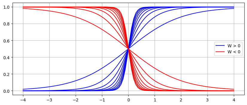
As \(W \to \infty\), the function \(\sigma(x; W,0)\) approaches the function

\[\begin{split} u(t) = \left\{ \begin{array}{ccc} 0 & , & t < 0 \\ 1/2 & , & t=0 \\ 1 & , & t > 0 \end{array} \right. \end{split}\]

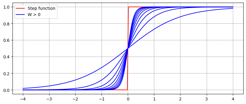
Use the function np.heaviside to plot the step function along with \(\sigma(x; W, 0)\) for several positive weight values \(W > 0\).

x = np.linspace(-4,4,200)
y = np.heaviside(x,1)
plt.figure(figsize=(10,4))
plt.plot(x,y,'r')
for W in np.arange(1,10):
    y = 1/(1 + np.exp(-W*x))
    plt.plot(x,y,'b')
plt.legend(['Step function','W > 0'])
plt.grid(True)
plt.show()

Similarly, as \(W \to -\infty\), the function \(\sigma(x; W,0)\) approaches the function

\[\begin{split} 1 - u(t) = \left\{ \begin{array}{ccc} 1 & , & t < 0 \\ 1/2 & , & t=0 \\ 0 & , & t > 0 \end{array} \right. \end{split}\]

How does \(b\) change the graph of the logistic function? Let \(W=1\) and plot \(\sigma(x;1,b)\) for many different values of \(b\).

N = 5
W = 1
x = N*np.linspace(-2,2,200)
plt.figure(figsize=(10,4))
for b in np.arange(-N,N+1):
    y = 1/(1 + np.exp(-(W*x + b)))
    plt.plot(x,y,'b',alpha=(b + N)/N/2)
plt.grid(True)
plt.show()

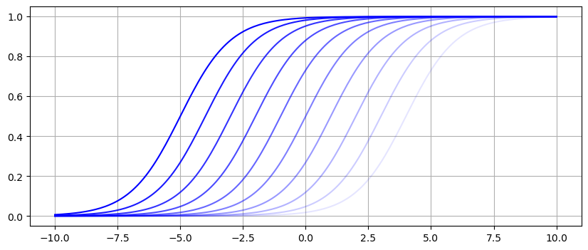
The bias parameters shifts the graph to the left by \(b/W\) since

\[ \sigma(x; W, b) = \frac{1}{1 + e^{-(Wx + b)}} = \frac{1}{1 + e^{-W(x + b/W)}} \]

See also

Check out Wikipedia: Logistic Function for more information.