Euler’s 3-Body Problem

import numpy as np
import matplotlib.pyplot as plt
import scipy.integrate as spi

Problem Statement

How does a planet move under the force of gravity due to two stars fixed in space?

See also

Check out Wikipedia: Euler’s 3-Body Problem for more information.

Variables and Parameters

Description	Symbol	Dimensions	Type
position of planet in \(x\)-direction	\(x\)	L	dependent variable
position of planet in \(y\)-direction	\(y\)	L	dependent variable
time	\(t\)	T	independent variable
mass of planet	\(m_p\)	M	parameter
mass of star 1	\(m_1\)	M	parameter
mass of star 2	\(m_2\)	M	parameter
gravitational constant	\(G\)	L3T-2M-1	parameter
distance of each star from the origin	\(d\)	L	parameter

Assumptions and Constraints

• planet moves in \(xy\)-plane only

• star 1 is located on the \(x\)-axis at \((-d,0)\)

• star 2 is located on the \(x\)-axis at \((+d,0)\)

Model Construction

The unit vector that points from the planet to star 1 is

\[ \left( -\frac{x+d}{\sqrt{(x+d)^2 + y^2}} , -\frac{y}{\sqrt{(x+d)^2 + y^2}} \right) \]

and the unit vector that points from the planet to star 2 is

\[ \left( -\frac{x-d}{\sqrt{(x-d)^2 + y^2}} , -\frac{y}{\sqrt{(x-d)^2 + y^2}} \right) \]

The sum of the gravitational forces of both stars acting on the planet is

\[\begin{split} \begin{align*} \mathbf{F} &= \frac{Gm_pm_1}{(x+d)^2 + y^2} \left( -\frac{x+d}{\sqrt{(x+d)^2 + y^2}} , -\frac{y}{\sqrt{(x+d)^2 + y^2}} \right) \\ & \quad \quad + \ \frac{Gm_pm_2}{(x-d)^2 + y^2} \left( -\frac{x-d}{\sqrt{(x-d)^2 + y^2}} , -\frac{y}{\sqrt{(x-d)^2 + y^2}} \right) \end{align*} \end{split}\]

Apply Newton’s second law of motion to get a second order, 2-dimenisional, nonlinear system of differential equations

\[\begin{split} \begin{align*} \frac{d^2x}{dt^2} &= -\frac{G m_1 (x+d)}{\left( (x+d)^2 + y^2 \right)^{3/2}} - \frac{G m_2 (x-d)}{\left( (x-d)^2 + y^2 \right)^{3/2}} \\ \frac{d^2y}{dt^2} &= -\frac{G m_1 y}{\left( (x+d)^2 + y^2 \right)^{3/2}} - \frac{G m_2 y}{\left( (x-d)^2 + y^2 \right)^{3/2}} \end{align*} \end{split}\]

with initial conditions

\[ x(0) = x_0 \ , \ \ y(0) = y_0 \ , \ \ x'(0) = v_{x,0} \ , \ \ y'(0) = v_{y,0} \ , \ \ \]

Apply nondimensionalization procedure. Let \(x = [x]x^*\), \(y = [y]y^*\) and \(t = [t]t^*\). It will simplify the equations greatly if we choose the same scaling factor \([c] = [x] = [y]\) for \(x\) and \(y\). Make the substitutions

\[\begin{split} \begin{align*} \frac{[c]}{[t]^2} \frac{d^2x^*}{dt^{*2}} &= -\frac{G m_1 ([c]x^* + d)}{\left( ([c]x^*+d)^2 + [c]^2y^{*2} \right)^{3/2}} - \frac{G m_2 ([c]x^*-d)}{\left( ([c]x^*-d)^2 + [c]^2y^{*2} \right)^{3/2}} \\ \frac{[c]}{[t]^2} \frac{d^2y^*}{dt^{*2}} &= -\frac{G m_1 [c]y^*}{\left( ([c]x^*+d)^2 + [c]^2y^{*2} \right)^{3/2}} - \frac{G m_2 [c]y^*}{\left( ([c]x^*-d)^2 + [c]y^{*2} \right)^{3/2}} \end{align*} \end{split}\]

Divide by highest order term and simplify

\[\begin{split} \begin{align*} \frac{d^2x^*}{dt^{*2}} &= -\frac{G m_1 [t]^2 (x^* + d^*)}{[c]^3 \left( (x^*+d^*)^2 + y^{*2} \right)^{3/2}} - \frac{G m_2 [t]^2 (x^*-d^*)}{[c]^3 \left( (x^*-d^*)^2 + y^{*2} \right)^{3/2}} \\ \frac{d^2y^*}{dt^{*2}} &= -\frac{G m_1 [t]^2 y^*}{[c]^3 \left( (x^*+d^*)^2 + y^{*2} \right)^{3/2}} - \frac{G m_2 [t]^2 y^*}{[c]^3 \left( (x^*-d^*)^2 + y^{*2} \right)^{3/2}} \end{align*} \end{split}\]

where \(d^* = d/[c]\). There are many choices and we choose \([c] = d\) and \([t] = \sqrt{\frac{d^3}{Gm_1}}\) and we arrive at

\[\begin{split} \begin{align*} \frac{d^2x^*}{dt^{*2}} &= -\frac{(x^* + 1)}{\left( (x^*+1)^2 + y^{*2} \right)^{3/2}} - \mu \frac{(x^*-1)}{\left( (x^*-1)^2 + y^{*2} \right)^{3/2}} \\ \frac{d^2y^*}{dt^{*2}} &= -\frac{y^*}{\left( (x^*+1)^2 + y^{*2} \right)^{3/2}} - \mu \frac{y^*}{\left( (x^*-1)^2 + y^{*2} \right)^{3/2}} \\ x^*(0) &= \frac{x_0}{d} \ , \ \ y^*(0) = \frac{y_0}{d} \\ \frac{dx^*}{dt^*}(0) &= v_{x,0} \sqrt{\frac{d}{Gm_1}} \ , \ \ \frac{dy^*}{dt^*}(0) = v_{y,0}\sqrt{\frac{d}{Gm_1}} \ , \ \ \end{align*} \end{split}\]

where \(\mu = \frac{m_2}{m_1}\).

Introduce new variables \(u_0 = x^*\), \(u_1 = \frac{dx}{dt^*}\), \(u_2 = y\), and \(u_3 = \frac{dy}{dt^*}\) to find

\[\begin{split} \begin{align*} \frac{du_0}{dt^*} &= u_1 \\ \frac{du_1}{dt^*} &= -\frac{(u_0 + 1)}{\left( (u_0+1)^2 + u_2^2 \right)^{3/2}} - \mu \frac{(u_0-1)}{\left( (u_0-1)^2 + u_2^2 \right)^{3/2}} \\ \frac{du_2}{dt^*} &= u_3 \\ \frac{du_3}{dt^*} &= -\frac{u_2}{\left( (u_0+1)^2 + u_2^2 \right)^{3/2}} - \mu \frac{u_2}{\left( (u_0-1)^2 + u_2^2 \right)^{3/2}} \end{align*} \end{split}\]

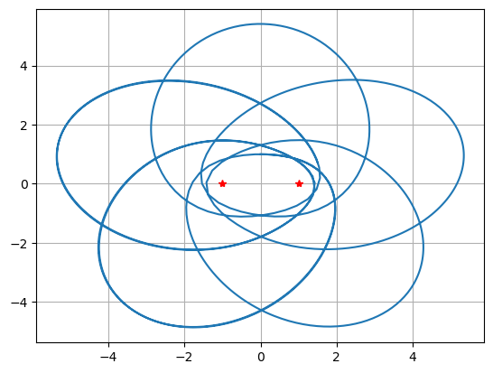
Plot some trajectories!

mu = 1.

def f(u,t):
    dudt = np.array([0.,0.,0.,0.])
    D1 = ((u[0] + 1)**2 + u[2]**2)**(3/2)
    D2 = ((u[0] - 1)**2 + u[2]**2)**(3/2)
    dudt[0] = u[1]
    dudt[1] = -(u[0] + 1)/D1 - mu*(u[0] - 1)/D2
    dudt[2] = u[3]
    dudt[3] = -u[2]/D1 - mu*u[2]/D2
    return dudt

u0 = [0.,1.5,1.,0.]
t = np.linspace(0,200,1000)
u = spi.odeint(f,u0,t)
plt.plot(u[:,0],u[:,2],-1,0,'r*',1,0,'r*'), plt.grid(True)
plt.show()

Analysis

Under construction