Global Energy Balance#
import numpy as np
import matplotlib.pyplot as plt
import scipy.integrate as spi
Problem Statement#
The Sun emits thermal radiation, a fraction of solar radiation is absorbed by the Earth and the rest is reflected into space, the Earth emits thermal radiation like a black body and some fraction of that thermal energy is absorbed by the atmosphere. Construct a mathematical model of the temperature of the Earth over time.
See also
Check out Mathematics and Climate > Chapter 2: Earth’s Energy Budget for more about climate models.
Variables and Parameters#
Description |
Symbol |
Dimensions |
Type |
|---|---|---|---|
temperature of the Earth and atmosphere |
\(T\) |
\(\Theta\) |
dependent variable |
time |
\(t\) |
T |
independent variable |
solar constant |
\(S_0\) |
M T-3 |
parameter |
albedo of the Earth |
\(\alpha\) |
1 |
parameter |
radius of the Earth |
\(R\) |
L |
parameter |
Stefan-Boltzmann constant |
\(\sigma\) |
M T-3 \(\Theta^{-4}\) |
parameter |
heat capacity of the Earth and atmosphere |
\(C\) |
M L2 T-2 \(\Theta^{-1}\) |
parameter |
greenhouse parameter |
\(\varepsilon\) |
1 |
parameter |
Assumptions and Constraints#
The Earth and the atmosphere form one object with homogeneous temperature \(T\) and heat capacity \(C\)
\(S_0\) is constant
Earth emits radiation as a black body \(\sigma T^4\)
\(\alpha\) is constant
\(C\) is constant
\(\varepsilon\) is constant
Construction#
The rate of energy absorbed by the Earth is \(Q_{in} = (1 - \alpha) \pi R^2 S_0\) and the rate of energy emitted by the Earth is \(Q_{out} = 4 \pi R^2 \sigma \varepsilon T^4\). The energy balance equation yields
Apply the nondimensionalization procedure. Let \(t = [t] t^*\) and \(T = [T] T^*\) and make the subtitution
Divide by the coefficient in \(T^4\) term
Choose values for scaling factors \([t]\) and \([T]\) to make coefficients equal to 1:
Rewrite the system:
Analysis#
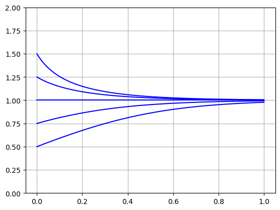
Since \(T>0\), there is only one steady state solution
The steady state depends only on the solar constant \(S_0\), albedo \(\alpha\), Stefan-Boltzmann constant \(\sigma\) and greenhouse parameter \(\varepsilon \). The parameters \(C\) and \(R\) only change the time scale \([t]\).
f = lambda T,t: 1 - T**4
t = np.linspace(0,1,100)

for T0 in [0.5,0.75,1.0,1.25,1.5]:
    T = spi.odeint(f,T0,t)
    plt.plot(t,T,'b')

plt.ylim([0,2]),plt.grid(True)
plt.show()