Residuals and $R^2$

import numpy as np
import matplotlib.pyplot as plt
import scipy.linalg as la
import pandas as pd

Residuals

Let $({\mathbf{x}}_1,y_1),\dots ,({\mathbf{x}}_N,y_N)$ be a data set of $N$ observations where each ${\mathbf{x}}_i=(x_{i,1},\dots ,x_{i,p})$ is a vector of values of the independent variables $x_1,\dots ,x_p$. Consider a linear regression model

$$y={\beta }_0+{\beta }_1{x}_1+\cdots +{\beta }_p{x}_p+\epsilon$$

where $\epsilon$ is the residual. Use the notation ${\epsilon }_i$ for the residual of the $i$th observation in the data set:

$${\epsilon }_i=y_i-({\beta }_0+{\beta }_1{x}_{i,1}+\cdots +{\beta }_p{x}_{i,p})$$

The parameters ${\beta }_0,{\beta }_1,\dots ,{\beta }_p$ are computed to minimize the residual sum of squares

$$RSS=\sum _{i=1}^N{\epsilon }_i^2$$

Once we compute parameters ${\beta }_0,\dots ,{\beta }_p$ which best fit the data, we would like to validate the model. We present two methods: the coefficient of determination $R^2$ (and $R_{adj}^2$) and graphical regression diagnostics.

Coefficient of Determination $R^2$

The quantity $RSS$ measures the total error of the linear regression model but the value on its own does not tell us how well the model fits the data. The coefficient of determination is given by

$$R^2=1-\frac{\sum _{i=1}^N{\epsilon }_i^2}{\sum _{i=1}^N(y_i-\overline{y}{)}^2}$$

The coefficient $R^2$ compares the error $RSS$ to the error of a model consisting of simply the mean value

$$\overline{y}=\frac{1}{N}\sum _{i=1}^N{y}_i$$

The value $R^2$ is near 1 when the model fits the data very closely and the value $R^2$ is near 0 when the linear regression model has nearly the same error as just simply drawing a straight horizontal line through the data. The definition of $R^2$ applies to any linear regression model however the value $RSS$ usually increases with the number of features $p$ in the model. Therefore we define the adjusted $R_{adj}^2$ coefficient as

$$R_{adj}^2=1-\frac{N-1}{N-p-1}\frac{\sum _{i=1}^N{\epsilon }_i^2}{\sum _{i=1}^N(y_i-\overline{y}{)}^2}$$

The coefficient $\frac{N-1}{N-p-1}$ takes into account the number of features in the model.

See also

Check out Wikipedia: Coefficient of Determination for more information.

Grapical Regression Diagnostics

The linear regression model is a good representation of the relationship between $y$ and $x_1,\dots ,x_p$ if the residual $\epsilon$ satisfies the following properties:

1. The residuals ${\epsilon }_i$ are normally distributed with mean 0.

2. Distribution of residuals ${\epsilon }_i$ does not depend on $x_1,\dots ,x_p$

3. Distribution of residuals ${\epsilon }_i$ does not depend on index $i$ (or time $t_i$)

We can verify these properties graphically by producing the following figures:

1. Plot histogram of residuals ${\epsilon }_i$

2. Plot ${\epsilon }_i$ versus $x_{i,j}$ for each feature $x_j$

3. Plot ${\epsilon }_i$ versus index $i$ (or time $t_i$)

Plot 1 should be a familiar bell curve centered at 0, and plots 2 and 3 should be random scatter plots with mean 0 and constant variance in the horizontal direction.

See also

Check out Wikipedia: Regression Validation for more information.

Example: REALTOR.ca

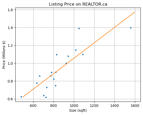
The data below was taken from REALTOR.ca for listings in the Kitsilano neighborhood of Vancouver. The variables $x_1,x_2,x_3$ correspond to the size (in square feet, sqft), the number of bedrooms and the number of bathrooms respectively. The dependent variable $y$ is the listing price.

x1 = np.array([1050,943,1557,662,829,724,482,702,733,637,819,802,771,779,823,924,1088,1018])
x2 = np.array([2,2,2,1,2,1,1,1,2,1,2,2,1,2,2,2,2,2])
x3 = np.array([2,2,2,1,2,1,1,1,1,1,1,1,1,2,2,2,2,2])
y  = np.array([1.39,1.079,1.398,0.859,1.098,0.619,0.625,0.639,0.728888,0.778,0.749888,0.825,0.858,0.899,0.8999,0.999888,1.099,1.149])

Let’s construct different linear regression models and compare the $R^2$ and $R_{adj}^2$ values. We’ll start with the model which includes only the size

$$y={\beta }_0+{\beta }_1{x}_1+\epsilon$$

Compute parameters ${\beta }_0,{\beta }_1$ and plot the result.

N = len(y)
X = np.column_stack([np.ones(N),x1])
beta = la.solve(X.T@X,X.T@y)
x1s = np.linspace(500,1600,50)
ys = beta[0] + beta[1]*x1s

plt.plot(x1,y,'.')
plt.plot(x1s,ys)
plt.title('Listing Price on REALTOR.ca')
plt.xlabel('Size (sqft)'), plt.ylabel('Price (Millons $)'), plt.grid(True)
plt.show()

Compute residuals and coefficient $R^2$.

residuals = y - (beta[0] + beta[1]*x1)
yhat = np.mean(y)
R2x1 = 1 - np.sum(residuals**2)/np.sum((y - yhat)**2)
print('R2 =',R2x1)

R2 = 0.7235562224127696

Repeat the procedure for the linear regression model $y={\beta }_0+{\beta }_1{x}_1+{\beta }_2{x}_2+\epsilon$.

X = np.column_stack([np.ones(N),x1,x2])
beta = la.solve(X.T@X,X.T@y)
residuals = y - (beta[0] + beta[1]*x1 + beta[2]*x2)
R2x1x2 = 1 - np.sum(residuals**2)/np.sum((y - yhat)**2)
R2adjx1x2 = 1 - (1 - R2x1x2)*(N - 1)/(N - 2 - 1)
print('R2 =',R2x1x2,'R2adj =',R2adjx1x2)

R2 = 0.7400376017871559 R2adj = 0.7053759486921101

Repeat the procedure again for the linear regression model $y={\beta }_0+{\beta }_1{x}_1+{\beta }_2{x}_2+{\beta }_3{x}_3+\epsilon$.

X = np.column_stack([np.ones(N),x1,x2,x3])
beta = la.solve(X.T@X,X.T@y)
residuals = y - (beta[0] + beta[1]*x1 + beta[2]*x2 + beta[3]*x3)
R2x1x2x3 = 1 - np.sum(residuals**2)/np.sum((y - yhat)**2)
R2adjx1x2x3 = 1 - (1 - R2x1x2x3)*(N - 1)/(N - 3 - 1)
print('R2 =',R2x1x2x3,'R2adj =',R2adjx1x2x3)

R2 = 0.8302699983155557 R2adj = 0.7938992836688891

The coefficient of determination increases when we include the number of bedrooms and bathrooms!

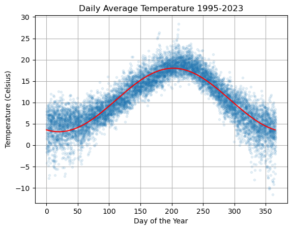
Example: Temperature

Let’s again look at daily average temperature in Vancouver (see vancouver.weatherstats.ca).

df = pd.read_csv('temperature.csv')

df.head()

	day	month	year	dayofyear	avg_temperature
0	13	4	2023	103	7.10
1	12	4	2023	102	5.19
2	11	4	2023	101	8.00
3	10	4	2023	100	7.69
4	9	4	2023	99	9.30

Let $T$ be the temperature and let $d$ be the day of the year. Define a regression model of the form

$$T={\beta }_0+{\beta }_1\cos (2\pi d/365)+{\beta }_2\sin (2\pi d/365)$$

Note that if we rewrite the variables as $y=T$, $x_1=\cos (2\pi d/365)$ and $x_2=\sin (2\pi d/365)$ then we see that this is indeed a linear regression model

$$y={\beta }_0+{\beta }_1{x}_1+{\beta }_2{x}_2$$

Construct the corresponding data matrix $X$ and compute the coefficient vector $\mathit{\beta }$.

N = len(df)
d = df['dayofyear']
T = df['avg_temperature']
X = np.column_stack([np.ones(N),np.cos(2*np.pi*d/365),np.sin(2*np.pi*d/365)])
beta = la.solve(X.T@X,X.T@T)

ds = np.linspace(0,365,500)
x1 = np.cos(2*np.pi*ds/365)
x2 = np.sin(2*np.pi*ds/365)
Ts = beta[0] + beta[1]*x1 + beta[2]*x2

plt.plot(df['dayofyear'],df['avg_temperature'],'.',alpha=0.1,lw=0)
plt.plot(ds,Ts,'r'), plt.grid(True)

plt.title('Daily Average Temperature 1995-2023')
plt.xlabel('Day of the Year'), plt.ylabel('Temperature (Celsius)')
plt.show()

Compute the residuals and plot the distribution:

f = lambda d,beta: beta[0] + beta[1]*np.cos(2*np.pi*d/365) + beta[2]*np.sin(2*np.pi*d/365)
residuals = T - f(d,beta)
plt.hist(residuals,bins=50,density=True), plt.grid(True)
plt.title('Distribution of Residuals')
plt.xlabel('Residual'), plt.ylabel('Relative Frequency')
plt.show()

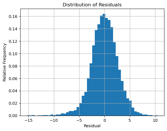
The distribution definitely looks like a normal distribution. Compute the mean and variance:

mean = np.mean(residuals)
var = np.var(residuals)
print('mean =',mean,', variance =',var)

mean = 2.8549607122840824e-14 , variance = 6.773167782960342

Compute the coefficients $R^2$ and $R_{adj}^2$:

That = np.mean(T)
R2 = 1 - np.sum(residuals**2)/np.sum((T - That)**2)
R2adj = 1 - (N-1)/(N-2-1)*np.sum(residuals**2)/np.sum((T - That)**2)
print('R2 =',R2,'R2adj =',R2adj)

R2 = 0.8035962434723157 R2adj = 0.8035569509332485

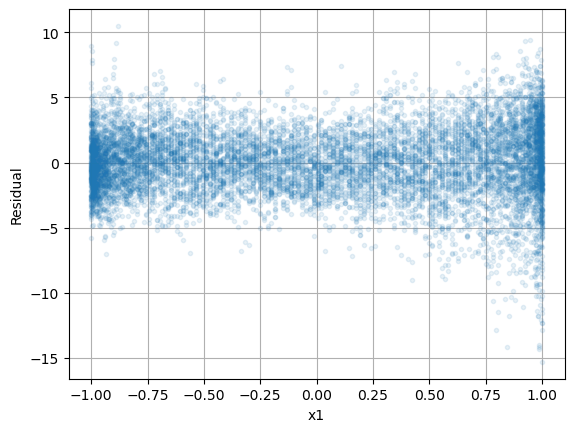
Next, let’s plot the residuals ${\epsilon }_i$ versus each of the input variables $x_1$ and $x_2$.

plt.plot(np.cos(2*np.pi*d/365),residuals,'.',alpha=0.1), plt.grid(True)
plt.xlabel('x1'), plt.ylabel('Residual')
plt.show()

plt.plot(np.sin(2*np.pi*d/365),residuals,'.',alpha=0.1), plt.grid(True)
plt.xlabel('$x_2$'), plt.ylabel('Residual')
plt.show()

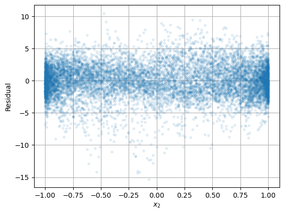
Both plots suggest that there is not much variation with respect to $x_1$ and $x_2$.

Now let’s plot ${\epsilon }_i$ versus day of the year $d$.

plt.plot(d,residuals,'.',alpha=0.1), plt.grid(True)
plt.xlabel('Day of the Year'), plt.ylabel('Residual')
plt.show()

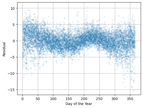
We can see there is some variation in the error! This means that our model is missing something. It looks like there is a variation with period 6 months. Let’s build that into the model!

Example: Temperature with Biannual Variation

We can see in the previous example that the linear model doesn’t quite fit the data. Let’s modify our linear regression model to include periodic functions with periods of 1 year (365 days) and 6 months (365/2 days):

$$T={\beta }_0+{\beta }_1\cos (2\pi d/365)+{\beta }_2\sin (2\pi d/365)+{\beta }_3\cos (4\pi d/365)+{\beta }_4\sin (4\pi d/365)$$

Construct the corresponding data matrix $X$ and compute the coefficient vector $\mathit{\beta }$.

N = len(df)
d = df['dayofyear']
T = df['avg_temperature']
X = np.column_stack([np.ones(N),
                     np.cos(2*np.pi*d/365),np.sin(2*np.pi*d/365),
                     np.cos(4*np.pi*d/365),np.sin(4*np.pi*d/365)])
beta = la.solve(X.T@X,X.T@T)

ds = np.linspace(0,365,500)
x1 = np.cos(2*np.pi*ds/365)
x2 = np.sin(2*np.pi*ds/365)
x3 = np.cos(4*np.pi*ds/365)
x4 = np.sin(4*np.pi*ds/365)
Ts = beta[0] + beta[1]*x1 + beta[2]*x2 + beta[3]*x3 + beta[4]*x4

plt.plot(df['dayofyear'],df['avg_temperature'],'.',alpha=0.1,lw=0)
plt.plot(ds,Ts,'r'), plt.grid(True)
plt.title('Daily Average Temperature 1995-2023')
plt.xlabel('Day of the Year'), plt.ylabel('Temperature (Celsius)')
plt.show()

Analyze the model. Plot the distribution of residuals:

f = lambda d,beta: beta[0] + beta[1]*np.cos(2*np.pi*d/365) + beta[2]*np.sin(2*np.pi*d/365) + beta[3]*np.cos(4*np.pi*d/365) + beta[4]*np.sin(4*np.pi*d/365)
residuals = T - f(d,beta)
plt.hist(residuals,bins=50,density=True), plt.grid(True)
plt.title('Distribution of Residuals')
plt.xlabel('Residual'), plt.ylabel('Relative Frequency')
plt.show()

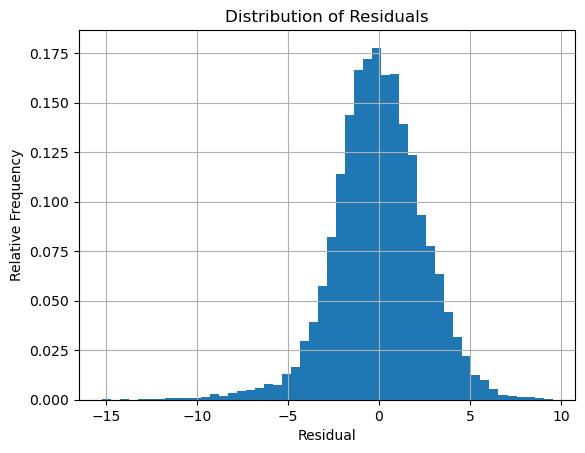
The distribution definitely looks like a normal distribution. Compute the mean and variance:

mean = np.mean(residuals)
var = np.var(residuals)
print('mean =',mean,', variance =',var)

mean = 2.6413715659145965e-14 , variance = 6.20105106178613

Compute the coefficients $R^2$ and $R_{adj}^2$:

That = np.mean(T)
R2 = 1 - np.sum(residuals**2)/np.sum((T - That)**2)
R2adj = 1 - (N-1)/(N-4-1)*np.sum(residuals**2)/np.sum((T - That)**2)
print('R2 =',R2,'R2adj =',R2adj)

R2 = 0.8201860987382082 R2adj = 0.8201141371969329

The coefficients both increase when we include the variables $x_3,x_4$.

Next, let’s plot the residuals ${\epsilon }_i$ versus each of the input variables $x_1,x_2,x_3,x_4$.

plt.subplot(2,2,1)
plt.plot(np.cos(2*np.pi*d/365),residuals,'.',alpha=0.1), plt.grid(True)
plt.xlabel('$x_1$'), plt.ylabel('Residual')

plt.subplot(2,2,2)
plt.plot(np.sin(2*np.pi*d/365),residuals,'.',alpha=0.1), plt.grid(True)
plt.xlabel('$x_2$'), plt.ylabel('Residual')

plt.subplot(2,2,3)
plt.plot(np.cos(4*np.pi*d/365),residuals,'.',alpha=0.1), plt.grid(True)
plt.xlabel('$x_3$'), plt.ylabel('Residual')

plt.subplot(2,2,4)
plt.plot(np.sin(4*np.pi*d/365),residuals,'.',alpha=0.1), plt.grid(True)
plt.xlabel('$x_4$'), plt.ylabel('Residual')

plt.tight_layout()
plt.show()

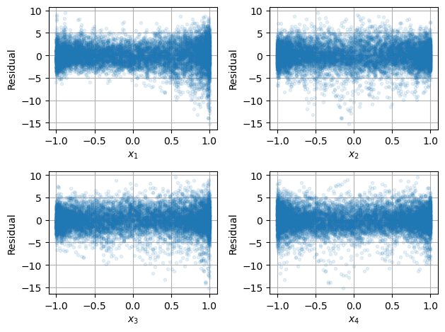
Finally, plot ${\epsilon }_i$ versus day of the year $d$.

plt.plot(d,residuals,'.',alpha=0.1), plt.grid(True)
plt.xlabel('Day of the Year'), plt.ylabel('Residual')
plt.show()

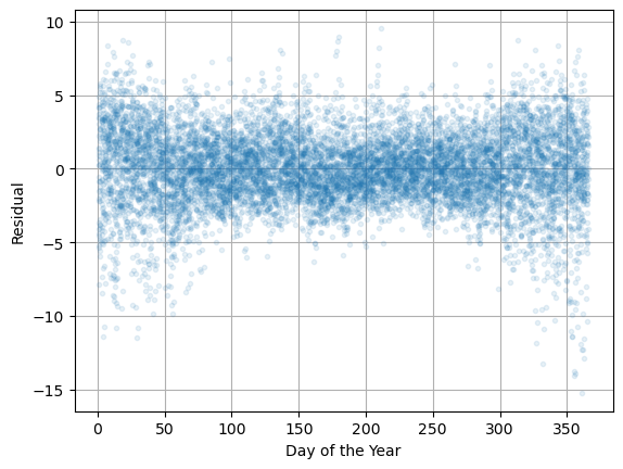
All the plots suggest the mean of the residual is 0 independent of each variable and time however the variance seems to increase in the winter. How can we account for this?