Conservation of Mass

import numpy as np
import matplotlib.pyplot as plt
import scipy.integrate as spi

Mass Balance Equation

The law of conservation of mass states that the mass of a closed system does not change. This implies that mass cannot be created or destroyed. Conservation of mass implies the balance equation for an open system

\[ \frac{dM}{dt} = Q_{\text{in}} - Q_{\text{out}} \]

where:

• \(M(t)\) is the mass in the system over time \(t\)

• \(Q_{in}\) is the mass flow rate into the system with dimensions MT^-1

• \(Q_{out}\) is the mass flow rate out of the system with dimensions MT^-1

See also

Check out Wikipedia: Conservation of Mass for more information.

Dilution

A tank contains a salt water solution. To dilute the solution, pure water is pumped into the tank and mixed. The solution is drained from the tank at the same rate as water is pumped into the tank. How does the concentration of the solution change over time?

Let’s define the variables and parameters in the model:

Description	Symbol	Dimensions	Type
mass of salt in the tank	\(M\)	M	dependent variable
time	\(t\)	T	independent variable
initial mass of salt in the tank	\(M_0\)	M	parameter
flow rate of fluid in/out of the tank	\(Q\)	L3T-1	parameter
volume of solution	\(V_0\)	L3	parameter

Note that the rate of salt flowing out of the tank is \(\frac{MQ}{V}\). Apply the mass balance equation to get

\[ \frac{dM}{dt} = -\frac{MQ}{V} \ , \ \ M(0) = M_0 \]

Apply the nondimensionalization procedure. Let \(t = [t]t^*\) and \(M = [M]M^*\) and make the substitution

\[ \frac{[M]}{[t]} \frac{dM^*}{dt^*} = -\frac{[M]M^* Q}{V} \ , \ \ [M]M^*(0) = M_0 \]

Choose \([t] = \frac{V}{Q}\) and \([M] = M_0\) and write

\[ \frac{dM^*}{dt^*} = -M^* \ , \ \ M^*(0) = 1 \]

Solve the equation to find \(M^*(t) = e^{-t^*}\). Equivalently, \(M(t) = M_0e^{-Qt/V}\).

Withdrawing from a Pension

The concept of mass transfer is very general! Consider the problem of withdrawing from a pension. A pension is a financial asset that earns interest and a retiree will withdraw funds from the pension for living expenses. Create a mathematical model of a retiree living on a pension.

Let’s define the variables and parameters in the model:

Description	Symbol	Dimensions	Type
total value of the pension	\(M\)	N	dependent variable
time	\(t\)	T	independent variable
rate of return	\(r\)	T-1	parameter
rate of withdrawal	\(w\)	NT-1	parameter

Assume that the rate of return and rate of withdrawal are constant. Apply the mass balance equation to get

\[ \frac{dM}{dt} = rM - w \ , \ \ M(0) = M_0 \]

Apply the nondimensionalization procedure. Let \(t = [t]t^*\) and \(M = [M]M^*\) and make the substitution

\[ \frac{[M]}{[t]} \frac{dM^*}{dt^*} = r[M]M^* - w \ , \ \ [M]M^*(0) = M_0 \]

Divide by the derivative coefficient

\[ \frac{dM^*}{dt^*} = r[t]M^* - \frac{w[t]}{[M]} \ , \ \ M^*(0) = \frac{M_0}{[M]} \]

Choose \([t] = 1/r\) and \([M] = w/r\) and write

\[ \frac{dM^*}{dt^*} = M^* - 1 \ , \ \ M^*(0) = M_0^* \]

where \(M_0^* = \frac{rM_0}{w}\).

Solve the equation to find \(M^*(t) = (M_0^* - 1)e^{t^*} + 1\). Equivalently,

\[ M(t) = \left( \frac{rM_0}{w} - 1 \right) e^{rt} + 1 \]

Two Tank System

Suppose two tanks are connected such that solution from each tank flows into the other at the same rate. Now suppose salt water solution is pumped into the first tank at a constant rate and solution from the second tank is pumped out of the tank and removed from the system at the same rate so that the total volume of solution in the two-tank system reamins constant. Create a mathematical model of the salt concentration in both tanks.

Let’s define the variables and parameters in the model:

Description	Symbol	Dimensions	Type
mass of salt tank 1	\(M_1\)	M	dependent variable
mass of salt tank 2	\(M_2\)	M	dependent variable
time	\(t\)	T	independent variable
salt concentration of solution flowing into tank 1	\(C\)	M L-3	parameter
flow rate of solution into tank 1	\(Q_1\)	L3T-1	parameter
flow rate of solution from tank 1 to tank 2	\(Q_0\)	L3T-1	parameter
volume of solution in tank 1	\(V_1\)	L3	parameter

Apply the mass balance equation to each tank to derive the equations

\[\begin{split} \begin{align*} \frac{dM_1}{dt} &= C Q_1 + \frac{M_2 Q_0}{V_2} - \frac{M_1 Q_0}{V_1} \\ \frac{dM_2}{dt} &= \frac{M_1 Q_0}{V_1} - \frac{M_2 Q_0}{V_2} - \frac{M_2 Q_1}{V_2} \end{align*} \end{split}\]

Apply the nondimensionalization procedure. Let \(t = [t]t^*\), \(M_1 = [M_1]M_1^*\) and \(M_2 = [M_2]M_2^*\) and make the substitution

\[\begin{split} \begin{align*} \frac{[M_1]}{[t]} \frac{dM_1^*}{dt^*} &= C Q_1 + \frac{[M_2] M_2^* Q_0}{V_2} - \frac{[M_1] M_1^* Q_0}{V_1} \\ \frac{[M_2]}{[t]} \frac{dM_2^*}{dt^*} &= \frac{[M_1]M_1^* Q_0}{V_1} - \frac{[M_2]M_2^* Q_0}{V_2} - \frac{[M_2]M_2^* Q_1}{V_2} \end{align*} \end{split}\]

Divide by the derivative coefficient in each equation

\[\begin{split} \begin{align*} \frac{dM_1^*}{dt^*} &= \frac{C Q_1 [t]}{[M_1]} + \frac{[t] [M_2] M_2^* Q_0}{[M_1] V_2} - \frac{[t] M_1^* Q_0}{V_1} \\ \frac{dM_2^*}{dt^*} &= \frac{[t] [M_1] M_1^* Q_0}{[M_2] V_1} - \frac{[t]M_2^* Q_0}{V_2} - \frac{[t]M_2^* Q_1}{V_2} \end{align*} \end{split}\]

There are 3 unknowns and 6 coefficients and so there are many choices. Let’s choose

\[ [t] = \frac{\sqrt{V_1 V_2}}{Q_0} \hspace{10mm} [M_1] = \frac{CQ_1 \sqrt{V_1V_2}}{Q_0} \hspace{10mm} [M_2] = \frac{CQ_1 V_2}{Q_0} \]

and then define the dimensionless parameters

\[ \nu = \sqrt{\frac{V_2}{V_1}} \hspace{20mm} \rho = \frac{Q_1}{Q_0} \]

Write the system in terms of the new dimensionless variables and parameters to get

\[\begin{split} \begin{align*} \frac{dM_1^*}{dt^*} &= 1 + M_2^* - \nu M_1^* \\ \frac{dM_2^*}{dt^*} &= M_1^* - \left(\frac{1 + \rho}{\nu} \right) M_2^* \end{align*} \end{split}\]

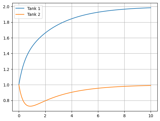
Plot some solutions:

nu = 1
rho = 1
f = lambda u,t: np.array([1 + u[1] - nu*u[0],u[0] - (1+rho)/nu*u[1]])
u0 = [1,1]
t = np.linspace(0,10,100)
u = spi.odeint(f,u0,t)
plt.plot(t,u[:,0],t,u[:,1])
plt.legend(['Tank 1','Tank 2']), plt.grid(True)
plt.show()