Gamma Distribution

import numpy as np
import matplotlib.pyplot as plt
import scipy.special as sps
import pandas as pd

Density Function

The gamma distribution (with parameters \(\alpha\) and \(\beta\)) is given by the probability density function

\[\begin{split} f(x) = \left\{ \begin{array}{ccc} \displaystyle \frac{\beta^{\alpha}}{\Gamma(\alpha)} x^{\alpha - 1} e^{-\beta x} & , & x \ge 0 \\ 0 & , & x < 0 \end{array} \right. \end{split}\]

where \(\Gamma\) is the Gamma function. We denote the gamma distribution by \(\Gamma(\alpha,\beta)\). Note that \(Exp(\lambda) = \Gamma(1,\lambda)\) The mean and variance are given by

\[ \mu = \frac{\alpha}{\beta} \hspace{1in} \sigma^2 = \frac{\alpha}{\beta^2} \]

Note that we can compute the parameters \(\alpha\) and \(\beta\) in terms of the mean and variance:

\[ \alpha = \frac{\mu^2}{\sigma^2} \hspace{1in} \beta = \frac{\mu}{\sigma^2} \]

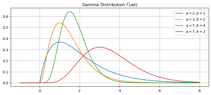
Let’s plot the gamma distrbution for different values of \(\alpha\) and \(\beta\). Use the function scipy.special.gamma to compute values of the gamma function \(\Gamma(x)\).

plt.figure(figsize=(10,4))
x = np.linspace(-1,8,1000)
gamma = lambda x,alpha,beta: beta**alpha/sps.gamma(alpha)*x**(alpha - 1)*np.exp(-beta*x)*np.heaviside(x,1)
for alpha,beta in [(2,1),(3,2),(7,4),(7,2)]:
    y = gamma(x,alpha,beta)
    plt.plot(x,y)
plt.title('Gamma Distribution $\Gamma(a b)$')
plt.legend(['$a=2,b=1$','$a=3,b=2$','$a=7,b=4$','$a=7,b=2$'])
plt.grid(True)
plt.show()

See also

Check out Wikipedia: Gamma Distribution for more information.

Example: Wind Speed Distribution

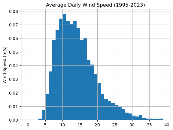
The file wind.csv consists of daily average wind speed measured at the Vancouver Airport from 1995 to 2023. Let’s import the data, look the first few rows and then plot the histogram of windspeeds.

df = pd.read_csv('wind.csv')
df.head()

	day	month	year	dayofyear	avg_wind_speed
0	13	4	2023	103	13.0
1	12	4	2023	102	13.0
2	11	4	2023	101	17.5
3	10	4	2023	100	11.5
4	9	4	2023	99	19.5

df['avg_wind_speed'].hist(bins=range(40),density=True)
plt.ylabel('Frequency'), plt.ylabel('Wind Speed (m/s)')
plt.title('Average Daily Wind Speed (1995-2023)')
plt.grid(True)
plt.show()

Compute the sample mean and sample variance.

mu = df['avg_wind_speed'].mean()
sigma2 = df['avg_wind_speed'].var()
print('mean =',mu,', variance =',sigma2)

mean = 13.9063 , variance = 33.23244355435653

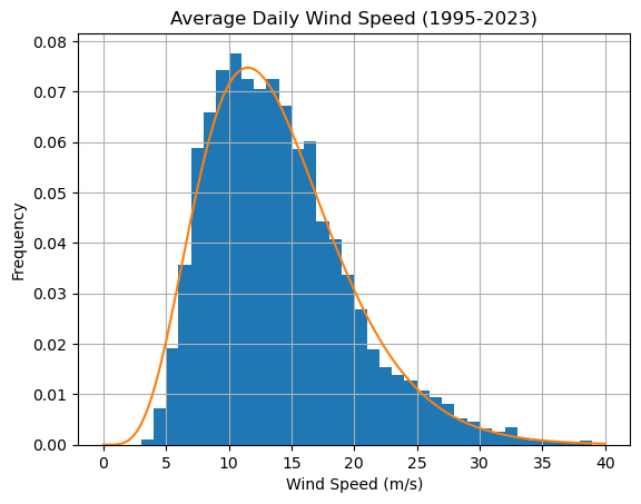
Compute the parameters \(\alpha\) and \(\beta\) and plot the distribution:

alpha = mu**2/sigma2
beta = mu/sigma2
df['avg_wind_speed'].hist(bins=range(40),density=True)
x = np.linspace(0,40,200)
y = gamma(x,alpha,beta)
plt.plot(x,y)
plt.xlabel('Wind Speed (m/s)'), plt.ylabel('Frequency')
plt.title('Average Daily Wind Speed (1995-2023)')
plt.grid(True)
plt.show()