Scalar Equations

import numpy as np
import scipy.integrate as spi
import matplotlib.pyplot as plt

Classification

A (scalar) differential equation is an equation involving an unknown function \(y(t)\) and its derivatives \(y',y'',y''',\dots\) There are many different kinds of differential equations and there are different methods to study and (hopefully) solve equations of different types and so the first step in analyzing a differential equation is to classify it.

The order of a differential equation is the highest order derivative of the unknown function \(y(t)\) appearing in the equation. For example, the equation

\[ y' = 1 - y \]

is a first order equation, and

\[ y'' + ty' + y = 1 \]

is a second order equation.

A first order equation is separable if it can be written in the form

\[ y' = f(t) g(y) \]

for some functions \(f(t)\) and \(g(y)\). For example, the equation

\[ y' = t \cos(y) \]

is separable, and the equation

\[ y' = t + y \]

is not separable.

A differential equation of order \(n\) is linear if it can be written in the form

\[ a_n(t) y^{(n)} + a_{n-1}(t) y^{(n-1)} + \cdots + a_1(t) y' + a_0(t) y = f(t) \]

where the coefficients \(a_n(t),a_{n-1}(t),\dots,a_0(t)\) are functions of the independent variable \(t\). For example, the equation

\[ t^2 y'' + t y' + y = \cos(t) \]

is a second order linear equation, and the equation

\[ y' = ty^2 \]

is a first order nonlinear equation.

A linear differential equation of order \(n\) is homogeneous if \(y(t) = 0\) is a solution. In other words, a linear homogeneous equation is of the form

\[ a_n(t) y^{(n)} + a_{n-1}(t) y^{(n-1)} + \cdots + a_1(t) y' + a_0(t) y = 0 \]

An essential property of linear homogeneous equations is superposition: if \(y_1(t)\) and \(y_2(t)\) are both solutions of the same linear homogeneous equation then \(y_1(t) + y_2(t)\) is also a solution since

\[\begin{split} \begin{align*} & a_n(t) (y_1 + y_2)^{(n)} + a_{n-1}(t) (y_1 + y_2)^{(n-1)} + \cdots + a_1(t) (y_1 + y_2)' + a_0(t) (y_1 + y_2) \\ &= a_n(t) y_1^{(n)} + a_n(t) y_2^{(n)} + a_{n-1}(t) y_1^{(n-1)} + a_{n-1}(t) y_2^{(n-1)} \\ & \quad \quad + \cdots + a_1(t) y_1' + a_1(t)y_2' + a_0(t) y_1 + a_0(t) y_2 \\ &= \left( a_n(t) y_1^{(n)} + a_{n-1}(t) y_1^{(n-1)} + \cdots + a_1(t) y_1' + a_0(t) y_1 \right) \\ & \quad \quad + \left( a_n(t) y_2^{(n)} + a_{n-1}(t) y_2^{(n-1)} + \cdots + a_1(t)y_2' + a_0(t) y_2 \right) \\ &= 0 + 0 = 0 \end{align*} \end{split}\]

A first order equation is autonomous if it can be written in the form

\[ y' = f(y) \]

for some function \(f(y)\). For example, the equation

\[ y' = 1 - y \]

is autonomous, and the equation

\[ y' = t + y \]

is not autonomous. Note that an autonomous equation is also separable.

See also

Check out Notes on Diffy Qs: Section 0.3 for more examples of classifying differential equations.

First Order Separable Equations

Let \(y' = f(t)g(y)\) be a first order separable equation. Divide both sides by \(g(y)\) and integrate (if possible) to find the general solution

\[ \int \frac{dy}{g(y)} = \int f(t) dt \]

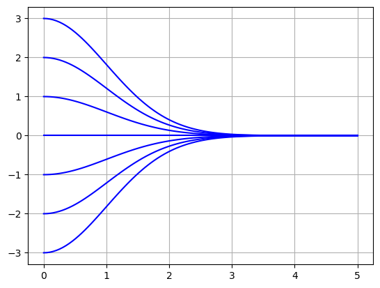
This is called the method of separation of variables. For example, consider the equation \(y' = -ty\) and compute

\[\begin{split} \begin{align*} \int \frac{dy}{y} &= -\int t dt \\ \ln |y| &= -\frac{t^2}{2} + C \\ y(t) &= k e^{-t^2/2} \end{align*} \end{split}\]

Plot the solution for different initial values \(y(0) = k\).

t = np.linspace(0,5,100)
for y0 in range(-3,4):
    y = y0*np.exp(-t**2/2)
    plt.plot(t,y,'b')
plt.grid(True)
plt.show()

See also

Check out Notes on Diffy Qs: Section 1.3 for more examples of first order separable equations.

Second Order Homogeneous Equations with Constant Coefficients

A second order homogeneous equation with constant coefficients is of the form

\[ ay'' + by' + cy = 0 \ \ , \ \ \ a,b,c \in \mathbb{R} \]

The characteristic polynomial of the equation is

\[ p(s) = as^2 + bs + c \]

and the roots of the characteristic polynomial

\[ r_1 = \frac{-b + \sqrt{b^2 - 4ac}}{2a} \hspace{20mm} r_2 = \frac{-b - \sqrt{b^2 - 4ac}}{2a} \]

determine the form of the general solution of the homogeneous equation.

If the roots are real and distinct (\(r_1 \ne r_2\)) then

\[ y(t) = C_1 e^{r_1 t} + C_2 e^{r_2 t} \ \ , \ \ \ C_1,C_2 \in \mathbb{R} \]

If the roots are real and repeated (\(r = r_1 = r_2\)) then

\[ y(t) = C_1 e^{r t} + C_2 t e^{r t} \ \ , \ \ \ C_1,C_2 \in \mathbb{R} \]

If the roots are complex conjugate then

\[ y(t) = C_1 e^{\alpha t} \cos(\beta t) + C_2 e^{\alpha t} \sin(\beta t) \ \ , \ \ \ C_1,C_2 \in \mathbb{R} \]

where \(r_1 = \alpha + i \beta\) and \(r_2 = \alpha - i \beta\) such that

\[ \alpha = -\frac{b}{2a} \hspace{20mm} \beta = \frac{\sqrt{4ac - b^2}}{2a} \]

See also

Check out Notes on Diffy Qs: Section 2.2 for more examples of second order homogeneous equations with constant coefficients.

Euler’s Method

Euler’s method is the simplest numerical method for approximating solutions of differential equations. Let \(y' = f(t,y)\), \(y(0) = y_0\), be a first order equation. Euler’s method is given by the recursive formula:

\[ y_{n+1} = y_n + h f(t_n,y_n) \]

where \(t_n = t_0 + nh\) for a chosen step size \(h\). Note that approximating the solution over the interval \([t_0,t_f]\) with \(N+1\) equally spaced points corresponds to step size

\[ h = \frac{t_f - t_0}{N} \]

Let’s write a Python function to implement Euler’s method:

def odeEuler(f,t,y0):
    y = np.zeros(len(t))
    y[0] = y0
    for n in range(0,len(t)-1):
        y[n+1] = y[n] + f(t[n],y[n])*(t[n+1] - t[n])
    return y

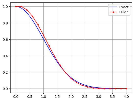
Let’s use Euler’s method to approximate the solution of \(y' = -ty\), \(y(0)=1\), over the interval \([0,4]\) with step size \(h=0.25\), and compare to the exact solution. Note that step size \(h = 0.25\) corresponds to \(N = 21\) in this case.

t_exact = np.linspace(0,4,100)
y_exact = np.exp(-t_exact**2/2)
plt.plot(t_exact,y_exact,'b')

f = lambda t,y: -t*y
y0 = 1
t = np.linspace(0,4,21)
y = odeEuler(f,t,y0)
plt.plot(t,y,'r.-')

plt.grid(True), plt.legend(['Exact','Euler'])
plt.show()

See also

Check out Notes on Diffy Qs: Section 1.7 for more about Euler’s method, and Mathematical Python: First Order Equations for more Python examples.

Numerical Solutions with SciPy

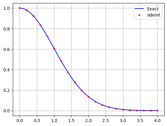
Euler’s method is simple to understand but it is not accurate enough to use in practice. The function scipy.integrate.odeint uses a higher order method to approximate solutions and it is what we use for real problems. Let’s use scipy.integrate.odeint to approximate the solution of \(y' = -ty\), \(y(0)=1\), and compare to the exact solution.

t_exact = np.linspace(0,4,100)
y_exact = np.exp(-t_exact**2/2)
plt.plot(t_exact,y_exact,'b')

f = lambda y,t: -t*y
y0 = 1
t = np.linspace(0,4,21)
y = spi.odeint(f,y0,t)
plt.plot(t,y,'r.')

plt.grid(True), plt.legend(['Exact','odeint'])
plt.show()

Note that the function odeint:

• automatically determines the step size at each step in its computation to guarantee a certain level of accuracy and so the input array t only specifies which values are returned. In particular, inputing more values in the vector t (ie. “smaller” step size \(h\)) does not increase the accuracy of the result. You can manually change the parameters atol and rtol.

• expects \(y\) as the first variable in the right hand side function \(f(y,t)\) in the equation \(y' = f(y,t)\).

See also

Check out Mathematical Python: Numerical Methods for more Python examples, and SciPy documentation for more information about scipy.integrate.odeint.