Planetary Orbits

import numpy as np
import matplotlib.pyplot as plt
import scipy.integrate as spi

Problem Statement

How does a planet move around a star under the force of gravity?

Variables and Parameters

Description	Symbol	Dimensions	Type
position of planet in \(x\)-direction	\(x\)	L	dependent variable
position of planet in \(y\)-direction	\(y\)	L	dependent variable
time	\(t\)	T	independent variable
mass of the planet	\(m_p\)	M	parameter
mass of the star	\(m_s\)	M	parameter
gravitational constant	\(G\)	L3T-2M-1	parameter

Assumptions and Constraints

• planet moves in the \(xy\)-plane only

• the position of the star is fixed at the origin

• no drag, friction or damping

• planet starts on the \(x\)-axis at \(y(0) = 0\)

• planet starts with velocity in \(y\)-direction only, \(x'(0) = 0\)

Model Construction

The unit vector that points from the planet to the star is

\[ \left( -\frac{x}{\sqrt{x^2 + y^2}} , -\frac{y}{\sqrt{x^2 + y^2}} \right) \]

The gravitational force vector acting on the planet is given by

\[ \mathbf{F} = \frac{Gm_pm_s}{x^2 + y^2} \left( -\frac{x}{\sqrt{x^2 + y^2}} , -\frac{y}{\sqrt{x^2 + y^2}} \right) \]

Apply Newton’s second law of motion to get a second order, 2-dimenisional, nonlinear system of differential equations

\[\begin{split} \begin{align*} m_p \frac{d^2x}{dt^2} &= -\frac{G m_p m_s x}{\left( x^2 + y^2 \right)^{3/2}} \\ m_p \frac{d^2y}{dt^2} &= -\frac{G m_p m_s y}{\left( x^2 + y^2 \right)^{3/2}} \end{align*} \end{split}\]

with initial conditions

\[ x(0) = x_0 \ , \ \ y(0) = 0 \ , \ \ x'(0) = v_{x,0} \ , \ \ y'(0) = v_{y,0} \ , \ \ \]

Apply nondimensionalization procedure. Let \(x = [x]x^*\), \(y = [y]y^*\) and \(t = [t]t^*\). The symmetry of the equations suggests that we should choose the same scaling factor \([c] = [x] = [y]\) for \(x\) and \(y\). Make the substitutions

\[\begin{split} \begin{align*} \frac{[c]}{[t]^2} \frac{d^2x^*}{dt^{*2}} &= -\frac{G m_s [c]x^*}{[c]^3 \left( x^{*2} + y^{*2} \right)^{3/2}} \\ \frac{[c]}{[t]^2} \frac{d^2y^*}{dt^{*2}} &= -\frac{G m_s [c]y^*}{[c]^3 \left( x^{*2} + y^{*2} \right)^{3/2}} \\ [c]x^*(0) &= x_0 \ , \ \ [c]y^*(0) = 0 \\ \frac{[c]}{[t]} \frac{dx^*}{dt^*}(0) &= 0 \ , \ \ \frac{[c]}{[t]} \frac{dy^*}{dt^*}(0) = v_{y,0} \end{align*} \end{split}\]

Divide by highest order term and simplify

\[\begin{split} \begin{align*} \frac{d^2x^*}{dt^{*2}} &= -\frac{G m_s [t]^2 x^*}{[c]^3 \left( x^{*2} + y^{*2} \right)^{3/2}} \\ \frac{d^2y^*}{dt^{*2}} &= -\frac{G m_s [t]^2y^*}{[c]^3 \left( x^{*2} + y^{*2} \right)^{3/2}} \\ x^*(0) &= \frac{x_0}{[c]} \ , \ \ y^*(0) = 0 \\ \frac{dx^*}{dt^*}(0) &= 0 \ , \ \ \frac{dy^*}{dt^*}(0) = \frac{[t]}{[c]} v_{y,0} \end{align*} \end{split}\]

There are several choices we can make and so we choose

\[ [c] = x_0 \hspace{10mm} \text{and} \hspace{10mm} [t] = \sqrt{ \frac{x_0^3}{Gm_s} } \]

and we get

\[\begin{split} \begin{align*} \frac{d^2x^*}{dt^{*2}} &= -\frac{x^*}{\left( x^{*2} + y^{*2} \right)^{3/2}} \\ \frac{d^2y^*}{dt^{*2}} &= -\frac{y^*}{\left( x^{*2} + y^{*2} \right)^{3/2}} \\ x^*(0) &= 1 \ , \ \ y^*(0) = 0 \\ \frac{dx^*}{dt^*}(0) &= 0 \ , \ \ \frac{dy^*}{dt^*}(0) = v_{y,0} \sqrt{\frac{x_0}{Gm_s}} \end{align*} \end{split}\]

Introduce new variables \(u_0 = x^*\), \(u_1 = \frac{dx}{dt^*}\), \(u_2 = y\), and \(u_3 = \frac{dy}{dt^*}\) to find

\[\begin{split} \begin{align*} \frac{du_0}{dt^*} &= u_1 \\ \frac{du_1}{dt^*} &= -\frac{u_0}{\left( u_0^2 + u_2^2 \right)^{3/2}} \\ \frac{du_2}{dt^*} &= u_3 \\ \frac{du_3}{dt^*} &= -\frac{u_2}{\left( u_0^2 + u_2^2 \right)^{3/2}} \end{align*} \end{split}\]

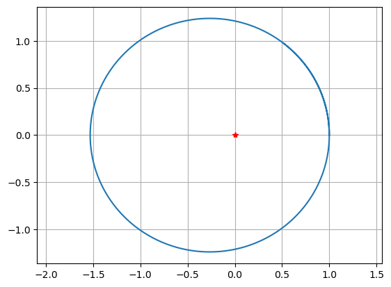
Plot some trajectories!

def f(u,t):
    dudt = np.array([0.,0.,0.,0.])
    d3 = np.sqrt(u[0]**2 + u[2]**2)**3
    dudt[0] = u[1]
    dudt[1] = -u[0]/d3
    dudt[2] = u[3]
    dudt[3] = -u[2]/d3
    return dudt

u0 = [1.,0.,0.,1.1]
t = np.linspace(0,10,200)
u = spi.odeint(f,u0,t)

plt.plot(u[:,0],u[:,2],0,0,'r*'), plt.grid(True), plt.axis('equal')
plt.show()

Analysis

Under construction