Cost and Regularization

import numpy as np
import matplotlib.pyplot as plt
import scipy.optimize as spo

Logistic Regression

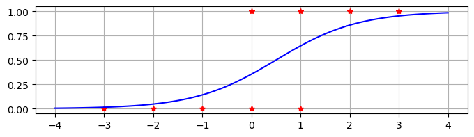
Suppose we have \(N\) data points \((x_0,y_0),\dots,(x_{N-1},y_{N-1})\) such that the targets are binary: \(y_k = 0\) or \(y_k = 1\) for \(k=0,\dots,N-1\). The goal of logistic regression is to find parameters \(W\) and \(b\) such that \(\sigma(x;W,b)\) “best fits” the data. Experiment with different values \(W\) and \(b\) to find a best fit line for the data below.

x = np.array([-3,-2,-1,0,0,1,1,2,3])
y = np.array([0,0,0,0,1,0,1,1,1])

W = 1.2
b = -0.6

sigma = lambda x: 1/(1 + np.exp(-(W*x + b)))
X = np.linspace(-4,4,100)
Y = sigma(X)

plt.figure(figsize=(8,2))
plt.plot(x,y,'r*',X,Y,'b'), plt.grid(True)
plt.show()

See also

Check out Wikipedia: Logistic Regression for more information.

Least Squares Cost Function

We need to define a cost function to find a line of “best fit”. We say that a model \(\sigma(x;W,b)\) best fits the data if the parameters minimize the cost function.

The mean least squares cost function is

\[ C_{LS}(W,b; x,y) = \frac{1}{N} \sum_{k=0}^{N-1} (y_k - \sigma(x_k; W,b) )^2 \]

Write a Python function called costLS which takes parameters W, b, x and y, and returns \(C_{LS}(W,b; x,y)\).

sigma = lambda x,W,b: 1/(1 + np.exp(-(W*x + b)))
costLS = lambda W,b,x,y: 1/len(x)*np.sum((y - sigma(x,W,b))**2)

Use the function to compute the cost for the data in the previous example with \(W=1.2\) and \(b=-1\). Try to modify the parameters \(W\) and \(b\) to minimize the cost.

x = np.array([-3,-2,-1,0,0,1,1,2,3])
y = np.array([0,0,0,0,1,0,1,1,1])
costLS(1.2,-1,x,y)

0.12963850207631072

Cross Entropy Cost Function

The cross entropy cost function:

\[ C_{CE}(W,b; x,y) = - \frac{1}{N} \sum_{k=0}^{N-1} \left( y_k \log(\sigma(x_k; W,b)) + (1 - y_k) \log(1 - \sigma(x_k; W,b)) \right) \]

Write a Python function called costCE which takes parameters W, b, x and y, and returns \(C_{CE}(W,b; x,y)\).

sigma = lambda x,W,b: 1/(1 + np.exp(-(W*x + b)))
costCE = lambda W,b,x,y: -1/len(y)*np.sum(y*np.log(sigma(x,W,b)) + (1 - y)*np.log(1 - sigma(x,W,b)))

Use the function to compute the cost for the data in the previous example with \(W=3\) and \(b=-1\). Try to modify the parameters \(W\) and \(b\) to minimize the cost.

x = np.array([-3,-2,-1,0,0,1,1,2,3])
y = np.array([0,0,0,0,1,0,1,1,1])
costCE(3,-1,x,y)

0.4340596605839115

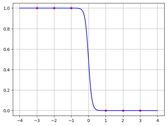
Regularization

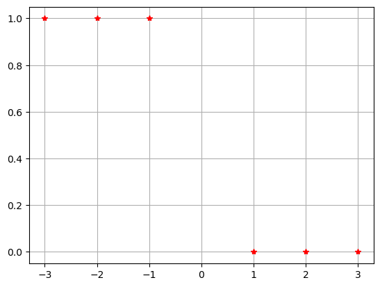
Consider the following example:

x = np.array([-3,-2,-1,1,2,3])
y = np.array([1,1,1,0,0,0])
plt.plot(x,y,'r*'), plt.grid(True)
plt.show()

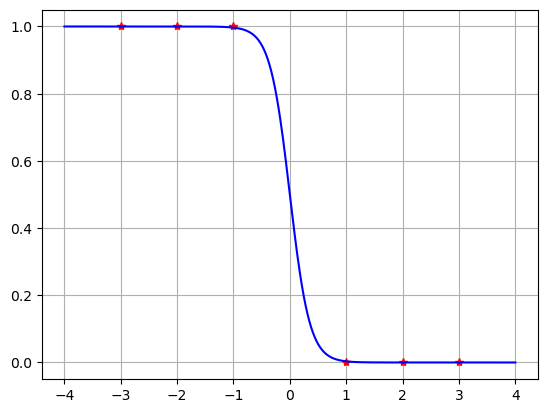
Because the data is separated, we can take the limit \(W \to \infty\) with \(b=0\) to get the step function which perfectly matches the data. However there is not a unique solution since we could allow any \(b\) such that \(-W < b < W\). And also we don’t want to consider infinite limits when doing mathematical computing.

W = -100
b = 50
costLS(W,b,x,y)

6.200126626701395e-45

X = np.linspace(-4,4,500)
Y = sigma(X,W,b)
plt.plot(x,y,'r*',X,Y,'b'), plt.grid(True)
plt.show()

Regularization adds a penalty for large values of the weight parameter \(W\). There are different ways to regularize such as \(L^2\) regularization, \(\alpha |W|^2\), and \(L^1\) regularization, \(\alpha |W|\), where \(\alpha\) is the regularization parameter.

Write a Python function called costCEL2 which takes parameters W, b, x, y and alpha, and returns the cross entropy cost function with \(L^2\) regularization:

\[ C_{CE}(W,b; x,y) = - \frac{1}{N} \sum_{k=0}^{N-1} \left( y_k \log(\sigma(x_k; W,b)) + (1 - y_k) \log(1 - \sigma(x_k; W,b)) \right) + \alpha |W|^2 \]

costCEL2 = lambda W,b,x,y,alpha: -1/len(y)*np.sum(y*np.log(sigma(x,W,b)) + (1 - y)*np.log(1 - sigma(x,W,b))) + alpha*np.abs(W)**2

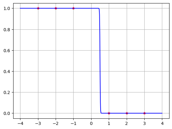
Use the function to compute the cost for the data in the previous example with \(W=-10\) and \(b=0\) and \(\alpha = 10^{-6}\). Try to modify the parameters \(W\) and \(b\) to minimize the cost.

x = np.array([-3,-2,-1,1,2,3])
y = np.array([1,1,1,0,0,0])
W = -10.3
b = 0
costCEL2(W,b,x,y,1e-6)

0.00011730122027635695

X = np.linspace(-4,4,500)
Y = sigma(X,W,b)
plt.plot(x,y,'r*',X,Y,'b'), plt.grid(True)
plt.show()

Computing Parameters with SciPy

Next time we will develop the gradient descent method to compute optimal parameters for logistic regression. Today let’s just use the function scipy.optimize.minimize takes a function \(F(\mathbf{z}) : \mathbb{R}^n \rightarrow \mathbb{R}\) and initial value \(\mathbf{z}_0\) can approximates a point \(\mathbf{c} \in \mathbb{R}^n\) such that \(F(\mathbf{c})\) is minimum.

In our case of fitting a logistic function to data using the cross entropy cost function with \(L^2\) regularization, we input the function

\[ F(\mathbf{z}) = C_{CE,L^2}(W,b; \mathbf{x},\mathbf{y}; \alpha) \]

where \(\mathbf{z} = [W,b]\). Use scipy.optimize.minimize to compute the optimal parameters for the example above.

F = lambda z: z[0]**2 + z[1]**2
result = spo.minimize(F,[1,1])

result

  message: Optimization terminated successfully.
  success: True
   status: 0
      fun: 2.311471135620994e-16
        x: [-1.075e-08 -1.075e-08]
      nit: 2
      jac: [-6.600e-09 -6.600e-09]
 hess_inv: [[ 7.500e-01 -2.500e-01]
            [-2.500e-01  7.500e-01]]
     nfev: 9
     njev: 3

alpha = 0.1
F = lambda z: costCEL2(z[0],z[1],x,y,alpha)
spo.minimize(F,[1,1])

  message: Optimization terminated successfully.
  success: True
   status: 0
      fun: 0.2626698735210554
        x: [-1.031e+00 -2.064e-05]
      nit: 9
      jac: [ 1.006e-07 -2.306e-06]
 hess_inv: [[ 1.910e+00 -2.590e-03]
            [-2.590e-03  8.234e+00]]
     nfev: 30
     njev: 10

x = np.array([-3,-2,-1,1,2,3])
y = np.array([1,1,1,0,0,0])

plt.plot(x,y,'r*'), plt.grid(True)
plt.show()

x = np.array([-3,-2,-1,1,2,3])
y = np.array([1,1,1,0,0,0])
alpha = 1e-4
F = lambda z: costCEL2(z[0],z[1],x,y,alpha)
result = spo.minimize(F,[1,1])

W = result.x[0]
b = result.x[1]
print("W =",W,"b =",b)

W = -5.680855932996707 b = -0.00016131134810909442

X = np.linspace(-4,4,500)
Y = sigma(X,W,b)
plt.plot(x,y,'r*',X,Y,'b'), plt.grid(True)
plt.show()