Multivariable Logistic Regression#
import numpy as np
import matplotlib.pyplot as plt
from sklearn.linear_model import LogisticRegression
from sklearn.datasets import load_iris
Multivariable Logistic Function#
The multivariable logistic function is
where \(\mathbf{x} \in \mathbb{R}^n\) and \(\mathbf{W} \in \mathbb{R}^n\) is the weight vector and \(b \in \mathbb{R}\) is the bias parameter. The term \(\langle \mathbf{W} , \mathbf{x} \rangle\) is the inner product
where
Halfspaces and Decision Boundary#
Fix a weight vector \(\mathbf{W} \in \mathbb{R}^n\) and bias parameter \(b \in \mathbb{R}\). The equation \(\langle \mathbf{W} , \mathbf{x} \rangle + b = 0\) defines a hyperplane
The space \(\mathbb{R}^n\) is divided into the halfspaces
and
Note that \(\sigma(\mathbf{x}; \mathbf{W},b) > 1/2\) for all \(\mathbf{x} \in H_+\) and \(\sigma(\mathbf{x}; \mathbf{W},b) < 1/2\) for all \(\mathbf{x} \in H_-\) therefore if we use the function \(\sigma(\mathbf{x}; \mathbf{W},b)\) as a logistic regression model for classification then the model predicts \(y=1\) for all \(\mathbf{x} \in H_+\) and \(y=0\) for all \(\mathbf{x} \in H_-\). The halfspaces are separated by \(H_0\) and so we call \(H_0\) the decision boundary.
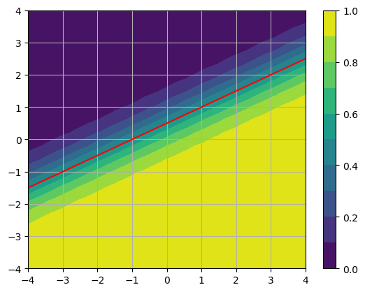
For example, let’s plot the logistic function for \(n=2\) with \(\mathbf{W} = (1,-2)^T\) and \(b = 1\) and include the decision boundary.
x0 = np.linspace(-4,4,20)
x1 = np.linspace(-4,4,20)
X0,X1 = np.meshgrid(x0,x1)
W0 = 1; W1 = -2; b = 1;
Y = 1/(1 + np.exp(-(W0*X0 + W1*X1 + b)))
plt.contourf(X0,X1,Y,levels=np.arange(0,1.1,0.1)), plt.colorbar()
plt.contour(X0,X1,Y,levels=[0.5],colors='r')
plt.grid(True)
plt.show()
Cross Entropy#
Let \((\mathbf{x}_0,y_0),\dots,(\mathbf{x}_{N-1},y_{N-1})\) be a set of observations such that \(\mathbf{x}_k \in \mathbf{R}^n\) and \(y_k = 0\) or \(1\) for all \(k=0,\dots,N-1\). The cross entropy cost function with L2 regularization is given by
We construct a logistic regression model for the data by computing optimal parameters \(\mathbf{W}\) and \(b\) which minimize \(C(\mathbf{W},b,\alpha)\) for a suitable choice of the regularization parameters \(\alpha\).
Computing Optimal Parameters with sklearn#
The function sklearn.linear_model.LogisticRegression computes optimal parameters \(\mathbf{W}\) and \(b\) using the cross entropy cost function. The function implements L2 regularization by default with regularization parameter \(C = 1\). Note that the parameter \(C\) corresponds to \(1/\alpha\) in our formulation.
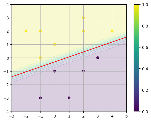
Consider the example data:
X = np.array([[2,3],[-1,2],[0,1],[1,-3],[4,2],[-1,-3],[3,0],[2,2],[2,-1],[-2,2],[-1,0],[0,-1]])
y = [1,1,1,0,1,0,0,1,0,1,1,0]
plt.scatter(X[:,0],X[:,1],c=y), plt.colorbar()
plt.grid(True)
plt.show()
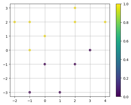
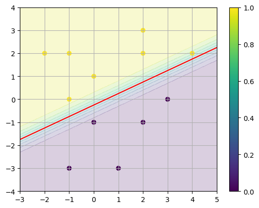
We can estimate the parameters \(\mathbf{W} = (-2,4)^T\) and \(b=1\) simply by inspection.
x0 = np.linspace(-3,5,50); x1 = np.linspace(-4,4,50);
X0,X1 = np.meshgrid(x0,x1)

W0 = -2; W1 = 4; b = 1
Y = 1/(1 + np.exp(-(W0*X0 + W1*X1 + b)))
plt.contourf(X0,X1,Y,levels=10,alpha=0.2)
plt.contour(X0,X1,Y,levels=[0.5],colors='r')

plt.scatter(X[:,0],X[:,1],c=y)
plt.grid(True), plt.colorbar()
plt.show()
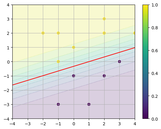
Now let’s use LogisticRegression to fit the model. First, let’s do the computation with \(C=1\).
model = LogisticRegression(C=1).fit(X,y)
The result is an object which we assign to the variable model.
type(model)
sklearn.linear_model._logistic.LogisticRegression
The object stores the model parameters as attributes. Access the weight vector \(\mathbf{W}\) by the attribute .coeff_.
model.coef_
array([[-0.46001636, 1.40410441]])
Access the bias parameter \(b\) by the attribute .intercept_.
model.intercept_
array([0.46965697])
x0 = np.linspace(-4,4,50); x1 = np.linspace(-4,4,50);
X0,X1 = np.meshgrid(x0,x1)

W0 = model.coef_[0,0]; W1 = model.coef_[0,1]; b = model.intercept_[0]
Y = 1/(1 + np.exp(-(W0*X0 + W1*X1 + b)))
plt.contourf(X0,X1,Y,levels=10,alpha=0.2)
plt.contour(X0,X1,Y,levels=[0.5],colors='r')

plt.scatter(X[:,0],X[:,1],c=y)
plt.grid(True), plt.colorbar()
plt.show()
Note that the classes \(y=0\) and \(y=1\) are clearly separated and so we can reduce the regularization parameter \(\alpha\) (increase \(C\)) to allow larger values \(\Vert \mathbf{W} \Vert\) which corresponds to a steeper step function from \(y=0\) to \(y=1\).
x0 = np.linspace(-3,5,50); x1 = np.linspace(-4,4,50);
X0,X1 = np.meshgrid(x0,x1)

model = LogisticRegression(C=100).fit(X,y)
W0 = model.coef_[0,0]; W1 = model.coef_[0,1]; b = model.intercept_[0]
Y = 1/(1 + np.exp(-(W0*X0 + W1*X1 + b)))
plt.contourf(X0,X1,Y,levels=10,alpha=0.2)
plt.contour(X0,X1,Y,levels=[0.5],colors='r')

plt.scatter(X[:,0],X[:,1],c=y)
plt.grid(True), plt.colorbar()
plt.show()
See also
Check out the sklearn documentation to learn more about the LogisticRegression model.
Example: Iris Data#
The module sklearn.datasets includes example datasets and the function load_iris loads an object which contains a data matrix with 150 samples and 4 features, and a target vector with 150 values. We save the data matix as X and the target vector as y in the cells below.
iris = load_iris()
X = iris.data
y = iris.target
X.shape
(150, 4)
y.shape
(150,)
The data consists of length measurements of different species of iris flowers:
iris.feature_names
['sepal length (cm)',
 'sepal width (cm)',
 'petal length (cm)',
 'petal width (cm)']
iris.target_names
array(['setosa', 'versicolor', 'virginica'], dtype='<U10')
There are 3 targets values in the dataset and so let’s combine the species versicolor and virginica into the same category so that our target values are \(y=0\) if the species is setosa and \(y=1\) if the species is versicolor or virginica. Modify the vector y so that the target value 2 is now 1.
y[y == 2] = 1
Let’s build a logistic regression model for the features sepal length and sepal width. Plot the data:
plt.scatter(X[:,0],X[:,1],c=y)
plt.xlabel(iris.feature_names[0])
plt.ylabel(iris.feature_names[1])
plt.grid(True), plt.colorbar()
plt.show()
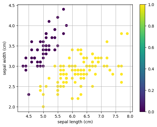
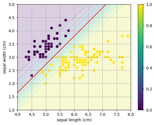
Use sklearn.linear_model.LogisticRegression to compute the logistic function. Note that LogisticRegression automatically applies L2 regularization with cross entropy cost function. The plot above shows that there is a clear separation between the two classes therefore reducing regularization will increase the weights to create a very sharp step function between the halfspaces. Adjust the parameter C in LogistRegression and observe the change in the logistic regression model.
model = LogisticRegression(C=1).fit(X[:,[0,1]],y)
W = model.coef_[0,:]
print('W =',W)
W = [ 3.38829757 -3.1645277 ]
b = model.intercept_[0]
print('b =',b)
b = -8.32330388643096
x0 = np.linspace(4,8,20); x1 = np.linspace(1,5,20);
X0,X1 = np.meshgrid(x0,x1)
Y = 1/(1 + np.exp(-(W[0]*X0 + W[1]*X1 + b)))
plt.contourf(X0,X1,Y,levels=10,alpha=0.2)
plt.contour(X0,X1,Y,levels=[0.5],colors='r')

plt.scatter(X[:,0],X[:,1],c=y)
plt.xlabel(iris.feature_names[0])
plt.ylabel(iris.feature_names[1])
plt.grid(True), plt.colorbar()
plt.show()
Let’s run the code again but increase the regularization parameter C (which corresponds to \(1/\alpha\) in our formulation).
model = LogisticRegression(C=100).fit(X[:,[0,1]],y)
W = model.coef_[0,:]
print('W =',W)
W = [ 11.95196336 -11.30095916]
b = model.intercept_[0]
print('b =',b)
b = -28.88900284027604
x0 = np.linspace(4,8,20); x1 = np.linspace(1,5,20);
X0,X1 = np.meshgrid(x0,x1)
Y = 1/(1 + np.exp(-(W[0]*X0 + W[1]*X1 + b)))
plt.contourf(X0,X1,Y,levels=10,alpha=0.2)
plt.contour(X0,X1,Y,levels=[0.5],colors='r')

plt.scatter(X[:,0],X[:,1],c=y)
plt.xlabel(iris.feature_names[0])
plt.ylabel(iris.feature_names[1])
plt.grid(True), plt.colorbar()
plt.show()
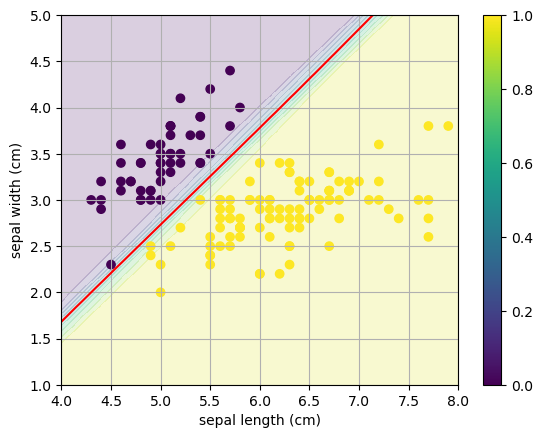
The weight vector defines the same decision boundary however the logistic function is a much sharper step function between the halfspaces.