2D Mass Spring System

import numpy as np
import scipy.integrate as spi
import matplotlib.pyplot as plt

Problem Statement

A flat object slides over a flat surface. The object is attached to one end of a spring and the spring is fixed at the other end. Construct a mathematical model of the motion of the object.

Variables and Parameters

Description	Symbol	Dimensions	Type
position of object in \(x\)-direction	\(x\)	L	dependent variable
position of object \(y\)-direction	\(y\)	L	dependent variable
time	\(t\)	T	independent variable
mass of the object	\(m\)	M	parameter
spring constant	\(k\)	MT-2	parameter
equilibrium length of the spring	\(L\)	L	parameter

Assumptions and Constraints

• no friction, drag or damping

• one end of the spring is fixed at the origin \((0,0)\) and the other end is attached to the mass a position \((x(t),y(t))\)

• the mass of the spring is negligible

Construction

The stretch/compression in the spring is the difference of the equilibrium length and the distance of the mass from origin. In other words, the stretch/compression in the spring is given by

\[ L - \| \mathbf{x}(t) \| \]

where \(\| \mathbf{x}(t) \| = \sqrt{ x(t)^2 + y(t)^2 }\). The spring force acts in the direction from the mass to the origin. The corresponding unit vector is

\[ \frac{\mathbf{x}(t)}{\| \mathbf{x}(t) \|} \]

Therefore the spring force is given by

\[ \mathbf{F}_s = k \left( L - \| \mathbf{x}(t) \| \right) \frac{\mathbf{x}(t)}{\| \mathbf{x}(t) \|} = k \left( \frac{L}{\| \mathbf{x}(t) \|} - 1 \right) \mathbf{x}(t) \]

Apply Newton’s second law of motion:

\[\begin{split} \begin{align*} m \frac{d^2x}{dt^2} &= \frac{k L x}{\sqrt{ x^2 + y^2 }} - k x \\ m \frac{d^2y}{dt^2} &= \frac{k L y}{\sqrt{ x^2 + y^2 }} - k y \end{align*} \end{split}\]

Apply the nondimensionalization procedure. Let \(x = [x]x^*\), \(y = [y]y^*\) and \(t = [t]t^*\). We should choose \([x] = [y]\) since there is no reason to treat the two directions differently and so let \([c] = [x] = [y]\). Make the substitutions:

\[\begin{split} \begin{align*} \frac{m[c]}{[t]^2} \frac{d^2 x^*}{dt^{*2}} &= \frac{k L [c]x^*}{[c] \sqrt{ x^{*2} + y^{*2} }} - k [c] x^* \\ \frac{m[c]}{[t]^2} \frac{d^2 y^*}{dt^{*2}} &= \frac{k L [c]y^*}{[c] \sqrt{ x^{*2} + y^{*2} }} - k [c] y^* \end{align*} \end{split}\]

Divide by the highest order coefficient \(m[c]/[t]^2\) to find:

\[\begin{split} \begin{align*} \frac{d^2 x^*}{dt^{*2}} &= \frac{k L [t]^2 x^*}{ m [c] \sqrt{ x^{*2} + y^{*2} }} - \frac{k [t]^2 x^*}{m} \\ \frac{d^2 y^*}{dt^{*2}} &= \frac{k L [t]^2 y^*}{ m [c] \sqrt{ x^{*2} + y^{*2} }} - \frac{k [t]^2 y^*}{m} \\ \end{align*} \end{split}\]

Choose scaling factors

\[ [t] = \sqrt{\frac{m}{k}} \hspace{20mm} [c] = L \]

and find

\[\begin{split} \begin{align*} \frac{d^2 x^*}{dt^{*2}} &= \frac{x^*}{ \sqrt{ x^{*2} + y^{*2} }} - x^* \\ \frac{d^2 y^*}{dt^{*2}} &= \frac{y^*}{ \sqrt{ x^{*2} + y^{*2} }} - y^* \end{align*} \end{split}\]

Introduce new variables

\[ u_0 = x^* \ , \ \ u_1 = \frac{dx^*}{dt^*} \ , \ \ u_2 = y^* \ , \ \ u_3 = \frac{dy^*}{dt^*} \]

and write the system as a first order system of equation

\[\begin{split} \begin{align*} \frac{du_0}{dt^*} &= u_1 \\ \frac{du_1}{dt^*} &= \frac{u_0}{ \sqrt{ u_0^2 + u_2^2 }} - u_0 \\ \frac{du_2}{dt^*} &= u_3 \\ \frac{du_3}{dt^*} &= \frac{u_2}{ \sqrt{ u_0^2 + u_2^2 }} - u_2 \end{align*} \end{split}\]

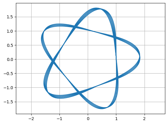
def f(u,t):
    dudt = np.array([0.,0.,0.,0.])
    D = np.sqrt(u[0]**2 + u[2]**2)
    dudt[0] = u[1]
    dudt[1] = u[0]/D - u[0]
    dudt[2] = u[3]
    dudt[3] = u[2]/D - u[2]
    return dudt

u0 = [1.,0.,0.,1.]
t = np.linspace(0,100,1000)
U = spi.odeint(f,u0,t)
plt.plot(U[:,0],U[:,2])
plt.grid(True), plt.axis('equal')
plt.show()

Analysis

Under construction