Exponential Distribution

import numpy as np
import matplotlib.pyplot as plt
import pandas as pd

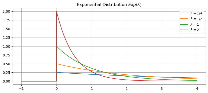
The exponential distribution (with parameter \(\lambda\)) is given by the probability density function

\[\begin{split} f(x) = \left\{ \begin{array}{ccc} \lambda e^{- \lambda x} & , & x \ge 0 \\ 0 & , & x < 0 \end{array} \right. \end{split}\]

We denote the exponential distribution by \(Exp(\lambda)\). The mean and variance are given by

\[ \mu = \frac{1}{\lambda} \hspace{1in} \sigma^2 = \frac{1}{\lambda^2} \]

Let’s plot the exponential distrbution for different values of \(\lambda\).

plt.figure(figsize=(10,4))
x = np.linspace(-1,4,1000)
exponential = lambda x,lam: lam*np.exp(-lam*x)*np.heaviside(x,1)
for lam in [.25,.5,1,2]:
    y = exponential(x,lam)
    plt.plot(x,y)
plt.title('Exponential Distribution $Exp(\lambda)$')
plt.legend(['$\lambda=1/4$','$\lambda=1/2$','$\lambda=1$','$\lambda=2$'])
plt.grid(True)
plt.show()

See also

Check out Wikipedia: Exponential Distribution for more information.

Example: Precipitation Data

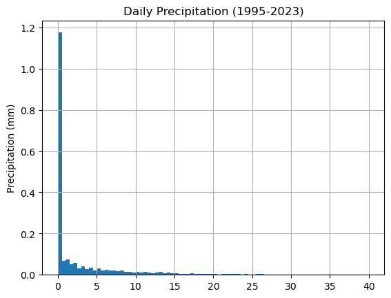
The file precipitation.csv consists of daily precipitation measured at the Vancouver Airport from 1995 to 2023. Let’s import the data, look the first few rows and then plot the histogram of precipitation.

df = pd.read_csv('precipitation.csv')
df.head()

	day	month	year	dayofyear	precipitation
0	13	4	2023	103	0.0
1	12	4	2023	102	0.0
2	11	4	2023	101	6.2
3	10	4	2023	100	0.0
4	9	4	2023	99	9.1

df['precipitation'].hist(bins=np.arange(0,40.5,0.5),density=True)
plt.ylabel('Frequency'), plt.ylabel('Precipitation (mm)')
plt.title('Daily Precipitation (1995-2023)')
plt.grid(True)
plt.show()

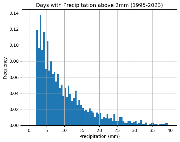
Let’s focus on days with at least 2mm of precipitation:

df = df[df['precipitation'] > 2]
df['precipitation'].hist(bins=np.arange(0,40.5,0.5),density=True)
plt.xlabel('Precipitation (mm)'), plt.ylabel('Frequency')
plt.title('Days with Precipitation above 2mm (1995-2023)')
plt.grid(True)
plt.show()

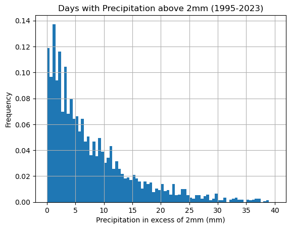
To fit an exponential distribution we need to shift the data:

df['precipitation2'] = df['precipitation'] - 2
df['precipitation2'].hist(bins=np.arange(0,40.5,0.5),density=True)
plt.xlabel('Precipitation in excess of 2mm (mm)'), plt.ylabel('Frequency')
plt.title('Days with Precipitation above 2mm (1995-2023)')
plt.grid(True)
plt.show()

Compute the sample mean and variance:

mu = df['precipitation2'].mean()
sigma2 = df['precipitation2'].var()
print('mean =',mu,', variance =',sigma2)

mean = 8.064954486345904 , variance = 71.13641043695192

The sample mean provides an estimate of the parameter \(\lambda\):

lam = 1/mu
print('lambda =',lam)

lambda = 0.12399326018429686

df['precipitation2'].hist(bins=np.arange(0,40.5,0.5),density=True)
x = np.linspace(0,40,200)
y = exponential(x,lam)
plt.plot(x,y)
plt.xlabel('Precipitation in excess of 2mm (mm)'), plt.ylabel('Frequency')
plt.title('Days with Precipitation above 2mm (1995-2023)')
plt.grid(True)
plt.show()

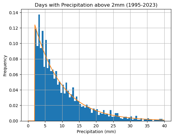
Finally, shift the data back again to better present the results:

df['precipitation'].hist(bins=np.arange(0,40.5,0.5),density=True)
x = np.linspace(0,40,400)
y = exponential(x-2,lam)
plt.plot(x,y)
plt.title('Days with Precipitation above 2mm (1995-2023)')
plt.xlabel('Precipitation (mm)'), plt.ylabel('Frequency')
plt.grid(True)
plt.show()