Gradient Descent

import numpy as np
import matplotlib.pyplot as plt

Directional Derivatives

Let $f(x_1,\dots ,x_n)$ be a differentiable function of several variables. Use vector notation to write the function as $f(\mathbf{x})$ where $\mathbf{x}\in {\mathbb{R}}^n$. The directional derivative of $f$ with respect to a unit vector $\mathbf{u}\in {\mathbb{R}}^n$ is

$$D_{\mathbf{u}}f(\mathbf{x})={\frac{d}{dt}(f(\mathbf{x}+t\mathbf{u}))|}_{t=0}$$

The value $D_{\mathbf{u}}f(\mathbf{x})$ is the slope of $f$ at $\mathbf{x}$ in the direction $\mathbf{u}$. Use the chain rule to compute

$$D_{\mathbf{u}}f(\mathbf{x})=\frac{\partial f}{\partial x_1}{u}_1+\cdots +\frac{\partial f}{\partial x_n}{u}_n$$

See also

Check out Wikipedia: Directional Derivative for more information.

Gradient Vector

The gradient of $f$ is

$$\mathrm{\nabla }f=(\frac{\partial f}{\partial x_1},\dots ,\frac{\partial f}{\partial x_n})$$

Therefore the directional derivative of $f$ with respect to $\mathbf{u}\in {\mathbb{R}}^n$ is the inner product

$$D_{\mathbf{u}}f(\mathbf{x})=\mathrm{\nabla }f\cdot \mathbf{u}=\frac{\partial f}{\partial x_1}{u}_1+\cdots +\frac{\partial f}{\partial x_n}{u}_n$$

This shows that the maximum value of $D_{\mathbf{u}}f(\mathbf{x})$ occurs when $\mathbf{u}$ points in the direction of the gradient $\mathrm{\nabla }f(\mathbf{x})$, and the minimum value occurs when $\mathbf{u}$ points in the opposite direction $-\mathrm{\nabla }f(\mathbf{x})$.

See also

Check out Wikipedia: Gradient for more information.

Gradient Descent

Suppose we want to minimize the function $f(\mathbf{x})$. Choose a starting point ${\mathbf{x}}_0\in {\mathbb{R}}^n$. The essential observation is that the function $f(\mathbf{x})$ decreases the fastest from the point ${\mathbf{x}}_0$ in the direction $-\mathrm{\nabla }f({\mathbf{x}}_{\mathbf{0}})$. Choose a step size $\alpha >0$ and define the next value ${\mathbf{x}}_1={\mathbf{x}}_0-\alpha \mathrm{\nabla }f({\mathbf{x}}_0)$. Repeat the process to generate a recursive sequence of points

$${\mathbf{x}}_{k+1}={\mathbf{x}}_k-\alpha \mathrm{\nabla }f({\mathbf{x}}_k)$$

The sequence ${\left\{{\mathbf{x}}_k\right\}}_{k=0}^{\mathrm{\infty }}$ should converge to a point $\mathbf{c}$ where $f(\mathbf{c})$ is a local minimum. The algorithm is called gradient descent.

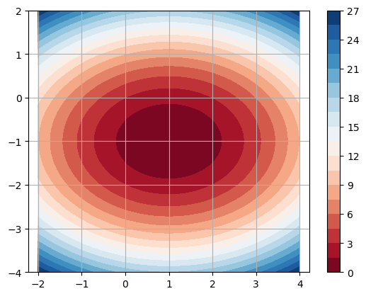
Let’s apply gradient descent to the function

$$f(x,y)=(x-1{)}^2+2(y+1{)}^2$$

The function is a paraboloid and the global minimum occurs at $(1,-1)$. Let’s plot the level curves of $f(x,y)$.

x = np.linspace(-2,4,50)
y = np.linspace(-4,2,50)
X,Y = np.meshgrid(x,y)
Z = (X - 1)**2 + 2*(Y + 1)**2
plt.contourf(X,Y,Z,levels=20,cmap='RdBu'), plt.colorbar()
plt.axis('equal'),plt.grid(True)
plt.show()

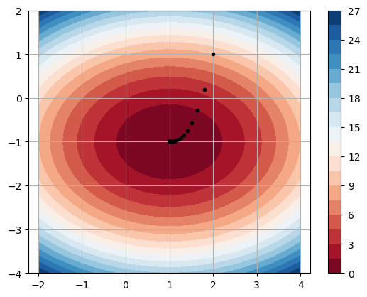
Compute the gradient

$$\mathrm{\nabla }f=(2x-2,4y+4)$$

and compute the sequence given by gradient descent starting from ${\mathbf{x}}_0=(2,1)$ with step size $\alpha =0.1$. Terminate the algorithm when $\Vert \mathrm{\nabla }f({\mathbf{x}}_k)\Vert <{10}^{-4}$.

x = np.linspace(-2,4,50)
y = np.linspace(-4,2,50)
X,Y = np.meshgrid(x,y)
Z = (X - 1)**2 + 2*(Y + 1)**2
plt.contourf(X,Y,Z,levels=20,cmap='RdBu'), plt.colorbar()

xk = np.array([2.,1.])
plt.plot(xk[0],xk[1],'k.')
alpha = 0.1
for k in range(100):
    grad = np.array([2*xk[0] - 2,4*xk[1] + 4])
    xk = xk - alpha*grad
    plt.plot(xk[0],xk[1],'k.')
    if np.linalg.norm(grad) < 1e-4:
        break

plt.axis('equal'),plt.grid(True)
plt.show()

Implementation

Let’s write a function called gradient_descent which takes input parameters:

• f is a vector function $f(\mathbf{x})$

• grad is the gradient $\mathrm{\nabla }f(\mathbf{x})$

• x0 is an initial point ${\mathbf{x}}_0\in {\mathbb{R}}^n$

• alpha is the step size

• max_iter is the maximum number of iterations

• eps is the stopping criteria $\Vert \mathrm{\nabla }f({\mathbf{x}}_k)\Vert <ϵ$

The function returns a $m\times n$ matrix X where row $k$ is the point

$${\mathbf{x}}_k={\mathbf{x}}_{k-1}-\alpha \mathrm{\nabla }f({\mathbf{x}}_{k-1})$$

The algorithm stops when $\Vert \mathrm{\nabla }f({\mathbf{x}}_k)\Vert <ϵ$ or the number of iterations exceeds max_iter. Therefore the number of rows of X is determined by the number of iterations completed. Let’s include default values alpha=0.1, max_iter=100 and eps=1e-4.

def gradient_descent(f,grad,x0,alpha=0.1,max_iter=100,eps=1e-4):
    X = np.zeros([max_iter+1,len(x0)])
    X[0,:] = x0
    for k in range(max_iter):
        xk = X[k,:]
        grad_xk = grad(xk)
        if np.linalg.norm(grad_xk) < eps:
            # Truncate the matrix X to include
            # only rows up to current index k
            X = X[:k+1,:]
            break
        X[k+1,:] = xk - alpha*grad_xk
    return X

Apply the function gradient_descent to the previous example.

f = lambda x: (x[0] - 1)**2 + 2*(x[1] + 1)**2
grad = lambda x: np.array([2*(x[0] - 1),4*(x[1] + 1)])
X = gradient_descent(f,grad,[2,1])

Check the first few iterations:

X[:5,:]

array([[ 2.    ,  1.    ],
       [ 1.8   ,  0.2   ],
       [ 1.64  , -0.28  ],
       [ 1.512 , -0.568 ],
       [ 1.4096, -0.7408]])

Check the last iterations:

X[-5:,:]

array([[ 1.00010634, -1.        ],
       [ 1.00008507, -1.        ],
       [ 1.00006806, -1.        ],
       [ 1.00005445, -1.        ],
       [ 1.00004356, -1.        ]])

Let’s see how many iterations were computed in total:

X.shape

(46, 2)

Check the norm of the gradient at the last iteration. It should be less than $ϵ={10}^{-4}$.

np.linalg.norm(grad(X[-1,:]))

8.711228593580309e-05

And the norm of the gradient at the second last iteration should be more than $ϵ={10}^{-4}$:

np.linalg.norm(grad(X[-2,:]))

0.00010889035742372364

It works as expected!

Example

Consider the function

$$f(x,y)=5x^2+4y^2+x^4+2y^4-10x^{2}y$$

Plot some levels curves of the function:

x = np.linspace(-4,4,50)
y = np.linspace(-2,3,50)
X,Y = np.meshgrid(x,y)
Z = 5*X**2 + 4*Y**2 + X**4 + 2*Y**4 - 10*X**2*Y
plt.contourf(X,Y,Z,levels=[-10,-5,-2,-1,0,1,2,5,10],cmap='RdBu'), plt.colorbar()
plt.grid(True)
plt.show()

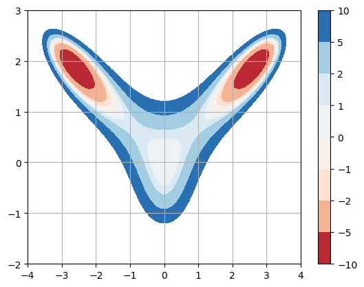
We see 5 critical points. Let’s approximate the local minimum near $(2.5,1.8)$. Compute the gradient

$$\mathrm{\nabla }f(x,y)=(10x+4x^3-20xy,8y+8y^3-10x^2)$$

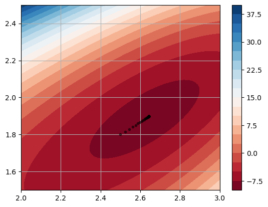
Apply gradient descent to $f(x,y)$.

f = lambda x: 5*x[0]**2 + 4*x[1]**2 + x[0]**4 + 2*x[1]**4 - 10*x[0]**2*x[1]
grad = lambda x: np.array([10*x[0] + 4*x[0]**3 - 20*x[0]*x[1], 8*x[1] + 8*x[1]**3 - 10*x[0]**2])
X = gradient_descent(f,grad,[2.5,1.8],0.01)

Inspect the first 5 points:

X[:5,:]

array([[2.5       , 1.8       ],
       [2.525     , 1.81444   ],
       [2.54485407, 1.82896844],
       [2.56201249, 1.84082887],
       [2.57638398, 1.85091924]])

And the last 5 points:

X[-5:,:]

array([[2.64421542, 1.89837822],
       [2.6442171 , 1.89837939],
       [2.64421847, 1.89838035],
       [2.64421957, 1.89838112],
       [2.64422047, 1.89838175]])

Plot all the points in the sequence to see it converge to the local minimum:

x = np.linspace(2,3,50)
y = np.linspace(1.5,2.5,50)
Xs,Ys = np.meshgrid(x,y)
Zs = 5*Xs**2 + 4*Ys**2 + Xs**4 + 2*Ys**4 - 10*Xs**2*Ys
plt.contourf(Xs,Ys,Zs,levels=20,cmap='RdBu'), plt.colorbar()
plt.plot(X[:,0],X[:,1],'k.',alpha=0.5)
plt.grid(True)
plt.show()

See also

Check out Wikipedia: Gradient Descent for more information.