Least Squares

import numpy as np
import matplotlib.pyplot as plt
import scipy.linalg as la
import pandas as pd

Residual Sum of Squares

Let \((\mathbf{x}_1,y_1),\dots,(\mathbf{x}_N,y_N)\) be a data set of \(N\) observations where each \(\mathbf{x}_i = (x_{i,1},\dots,x_{i,p})\) is a vector of values of the independent variables \(x_1,\dots,x_p\). Consider a linear regression model

\[ y = \beta_0 + \beta_1 x_1 + \cdots + \beta_p x_p + \varepsilon \]

The residual sum of squares is the cost function

\[ RSS = \sum_{i=1}^N |y_i - (\beta_0 + \beta_1 x_{i,1} + \cdots + \beta_p x_{i,p}) |^2 \]

The goal of least squares linear regression is to compute parameters \(\beta_0,\beta_1,\dots,\beta_p\) which minimize \(RSS\).

Normal Equations

Note that the expression for \(RSS\) above can be written in vector form using matrix multiplication

\[ RSS = || \mathbf{y} - X \boldsymbol{\beta} ||^2 \]

where

\[\begin{split} \mathbf{y} = \begin{bmatrix} y_1 \\ y_2 \\ \vdots \\ y_N \end{bmatrix} \hspace{20mm} X = \begin{bmatrix} 1 & x_{1,1} & \cdots & x_{1,p} \\ 1 & x_{2,1} & \cdots & x_{2,p} \\ \vdots & \vdots & \ddots & \vdots \\ 1 & x_{N,1} & \cdots & x_{N,p} \end{bmatrix} \hspace{20mm} \boldsymbol{\beta} = \begin{bmatrix} \beta_0 \\ \beta_1 \\ \vdots \\ \beta_p \end{bmatrix} \end{split}\]

The vector \(\boldsymbol{\beta}\) which minimizes \(RSS\) is the unique solution of the normal equations

\[ X^T X \boldsymbol{\beta} = X^T \mathbf{y} \]

Let’s see why this is true. Note that \(X \boldsymbol{\beta}\) is a vector in the column space of \(X\) therefore the distance \(|| \mathbf{y} - X \boldsymbol{\beta} ||\) is minimized when the line from \(\mathbf{y}\) to \(X\boldsymbol{\beta}\) is orthogonal to the column space of \(X\). In other words, we want to find \(\boldsymbol{\beta}\) such that \(\mathbf{y} - X \boldsymbol{\beta}\) is in the nullspace of \(X^T\) which leads to the equation \(X^T(\mathbf{y} - X \boldsymbol{\beta}) = 0\) and finally \(X^T X \boldsymbol{\beta} = X^T \mathbf{y}\).

Example: Real Estate Prices

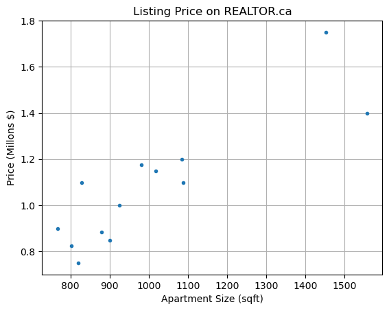
The data below was collected from REALTOR.ca for 2-bedroom apartments for sale in the Kitsilano neighborhood of Vancouver. The dependent variable \(y\) is the listing price and the independent variable \(x\) is the apartment size (in square feet).

x = [1557,1452,767,900,1018,802,924,981,879,819,829,1088,1085]
y = [1.398,1.750,0.899,0.848,1.149,0.825,0.999888,1.175,0.885,0.749888,1.098,1.099,1.198]
plt.plot(x,y,'.')
plt.title('Listing Price on REALTOR.ca')
plt.xlabel('Apartment Size (sqft)'), plt.ylabel('Price (Millons $)'), plt.grid(True)
plt.show()

Choose a simple linear regression model for the data \(y = \beta_0 + \beta_1 x + \varepsilon\). Construct the matrix \(X\):

X = np.column_stack([np.ones(len(x)),x])
X

array([[1.000e+00, 1.557e+03],
       [1.000e+00, 1.452e+03],
       [1.000e+00, 7.670e+02],
       [1.000e+00, 9.000e+02],
       [1.000e+00, 1.018e+03],
       [1.000e+00, 8.020e+02],
       [1.000e+00, 9.240e+02],
       [1.000e+00, 9.810e+02],
       [1.000e+00, 8.790e+02],
       [1.000e+00, 8.190e+02],
       [1.000e+00, 8.290e+02],
       [1.000e+00, 1.088e+03],
       [1.000e+00, 1.085e+03]])

Solve the normal equations:

beta = la.solve(X.T@X,X.T@y)
beta

array([0.10620723, 0.00096886])

Plot the linear regression model with the data:

xs = np.linspace(700,1600)
ys = beta[0] + beta[1]*xs
plt.plot(x,y,'.',xs,ys)
plt.title('Listing Price on REALTOR.ca'), plt.grid(True)
plt.xlabel('Apartment Size (sqft)'), plt.ylabel('Price (Millons $)')
plt.show()

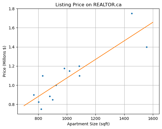
The coefficient \(\beta_1 = 0.00096886\) suggests that the listing price of a 2-bedroom apartment increases by \(968.86\) dollars per square foot.

Example: Temperature

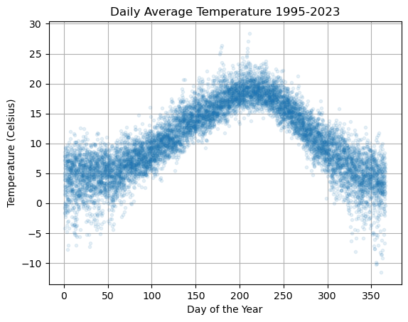
The file temperature.csv includes daily average temperature measured at the Vancouver Airport from 1995 to 2023 (see vancouver.weatherstats.ca). Let’s import the data, look the first few rows and then plot the average tempearture versus day of the year.

df = pd.read_csv('temperature.csv')

df.head()

	day	month	year	dayofyear	avg_temperature
0	13	4	2023	103	7.10
1	12	4	2023	102	5.19
2	11	4	2023	101	8.00
3	10	4	2023	100	7.69
4	9	4	2023	99	9.30

df.tail()

	day	month	year	dayofyear	avg_temperature
9995	1	12	1995	335	6.40
9996	30	11	1995	334	9.15
9997	29	11	1995	333	11.50
9998	28	11	1995	332	9.75
9999	27	11	1995	331	6.90

plt.plot(df['dayofyear'],df['avg_temperature'],'.',alpha=0.1,lw=0)
plt.title('Daily Average Temperature 1995-2023')
plt.xlabel('Day of the Year'), plt.ylabel('Temperature (Celsius)'), plt.grid(True)
plt.show()

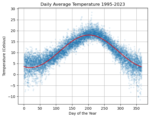
Let \(T\) by the temperature and let \(d\) be the day of the year. Define a regression model of the form

\[ T = \beta_0 + \beta_1 \cos(2 \pi d/365) + \beta_2 \sin(2 \pi d/365) \]

Note that if we rewrite the variables as \(y = T\), \(x_1 = \cos(2 \pi d/365)\) and \(x_2 = \sin(2 \pi d/365)\) then we see that this is indeed a linear regression model

\[ y = \beta_0 + \beta_1 x_1 + \beta_2 x_2 \]

Construct the corresponding data matrix \(X\) and compute the coefficient vector \(\boldsymbol{\beta}\).

N = len(df)
d = df['dayofyear']
T = df['avg_temperature']
X = np.column_stack([np.ones(N),np.cos(2*np.pi*d/365),np.sin(2*np.pi*d/365)])
beta = la.solve(X.T@X,X.T@T)

ds = np.linspace(0,365,500)
Ts = beta[0] + beta[1]*np.cos(2*np.pi*ds/365) + beta[2]*np.sin(2*np.pi*ds/365)

plt.plot(df['dayofyear'],df['avg_temperature'],'.',alpha=0.1,lw=0)
plt.plot(ds,Ts,'r'), plt.grid(True)

plt.title('Daily Average Temperature 1995-2023')
plt.xlabel('Day of the Year'), plt.ylabel('Temperature (Celsius)')
plt.show()