Systems of Equations

import numpy as np
import scipy.integrate as spi
import scipy.linalg as la
import matplotlib.pyplot as plt

Classification

A system of differential equations is a collection of equations involving unknown functions \(y_0(t),\dots,y_{d-1}(t)\) (with the same independent variable \(t\)) and their derivatives. The dimension of a system of differential equations is the number \(d\) of unknown functions \(y_0,\dots,y_{d-1}\) in the system. The order of a system of differential equations is the highest order derivative of any of the unknown functions appearing in the system. A system of differential equations is linear if each equation in the system is linear. A system of differential equations is autonomous if each equation in the system is autonomous.

For example, the system of differential equations

\[\begin{split} \begin{align*} x' &= x - xy \\ y' &= xy - y \end{align*} \end{split}\]

is a first order, 2-dimensional, autonomous, nonlinear system of differential equations, and the system

\[\begin{split} \begin{align*} x'' &= x - y \\ y' &= x - t \end{align*} \end{split}\]

is a second order, 2-dimensional, nonautonomous, linear system of differential equations.

See also

Check out Notes on Diffy Qs: Section 3.1 for more information about systems of differential equations.

First Order Transformation

A first order, \(d\)-dimensional system of differential equations is of the form

\[\begin{split} \begin{align*} u_0' &= f_0(t,u_0,\dots,u_{d-1}) \\ u_1' &= f_1(t,u_0,\dots,u_{d-1}) \\ & \ \ \vdots \\ u_{d-1}' &= f_{d-1}(t,u_0,\dots,u_{d-1}) \\ \end{align*} \end{split}\]

for some functions \(f_0,\dots,f_{d-1}\). Introduce vector notation

\[ \frac{d \mathbf{u}}{dt} = \mathbf{f}(t,\mathbf{u}) \]

where

\[\begin{split} \mathbf{u}(t) = \begin{bmatrix} u_0(t) \\ \vdots \\ u_{d-1}(t) \end{bmatrix} \hspace{10mm} \frac{d \mathbf{u}}{dt} = \begin{bmatrix} u_0'(t) \\ \vdots \\ u_{d-1}'(t) \end{bmatrix} \hspace{10mm} \mathbf{f}(t,\mathbf{u}) = \begin{bmatrix} f_0(t,u_0,\dots,u_{d-1}) \\ \vdots \\ f_{d-1}(t,u_0,\dots,u_{d-1}) \end{bmatrix} \end{split}\]

Any system of differential equations can be written as a first order system by introducing new variables. The procedure is as follows:

1. Identify the order of each unknown function in the system.

2. If \(y\) has order \(n\) then introduce \(n-1\) new variables for \(y\) and its derivatives: \(u_0 = y, u_1 = y',\dots,u_{n-1} = y^{(n-1)}\).

3. Rewrite the equations for \(u_0',\dots,u_{n-1}'\) in terms of the new variables only.

For example, consider a 1-dimensional, second order, linear equation with constant coefficients

\[ ay'' + by' + cy = f(t) \ \ , \ \ \ a,b,c \in \mathbb{R} \]

There is only one unknown function \(y\) and it has order 2 therefore we introduce \(u_0 = y\) and \(u_1 = y'\) and write

\[\begin{split} \begin{align*} u_0' &= u_1 \\ u_1' &= \frac{1}{a} \left( f(t) - bu_1 - cu_0 \right) \end{align*} \end{split}\]

Let’s try another example. Consider the following the system

\[\begin{split} \begin{align*} x'' &= 1 - y \\ y'' &= 1 - x \end{align*} \end{split}\]

Both \(x\) and \(y\) are second order therefore we introduce new variables \(u_0 = x, u_1 = x', u_2 = y, u_3 = y'\) and write

\[\begin{split} \begin{align*} u_0' &= u_1 \\ u_1' &= 1 - u_2 \\ u_2' &= u_3 \\ u_3' &= 1 - u_0 \end{align*} \end{split}\]

See also

Check out Notes on Diffy Qs: Section 3.1 for more examples of transforming higher order systems into first order systems.

Euler’s Method for Systems

We have seen numerical methods for first order scalar equations. How do we apply these methods to systems? First, transform the system into a first order system and then apply the method to each equation in the system simultaneously.

For example, let’s apply Euler’s method to a 2-dimensional, first order system

\[\begin{split} \begin{align*} x' &= f_1(t,x,y) \\ y' &= f_2(t,x,y) \end{align*} \end{split}\]

Starting with initial values \(x_0 = x(t_0)\) and \(y_0 = y(t_0)\) we define the resursive sequences

\[\begin{split} \begin{align*} x_{n+1} &= x_n + h f_1(t_n,x_n,y_n) \\ y_{n+1} &= y_n + h f_2(t_n,x_n,y_n) \end{align*} \end{split}\]

where \(t_n = t_0 + nh\) for step size \(h\). Use vector notation to write

\[ \mathbf{u}_{n+1} = \mathbf{u}_n + h \, \mathbf{f}(t_n,\mathbf{u}_n) \]

where

\[\begin{split} \mathbf{u}_n = \begin{bmatrix} x_n \\ y_n \end{bmatrix} \end{split}\]

Let’s write a function to implement Euler’s method for systems:

def odeEulerSys(f,t,u0):
    u = np.zeros([len(t),len(u0)])
    u[0,:] = u0
    for n in range(0,len(t)-1):
        u[n+1,:] = u[n,:] + f(t[n],u[n,:])*(t[n+1] - t[n])
    return u

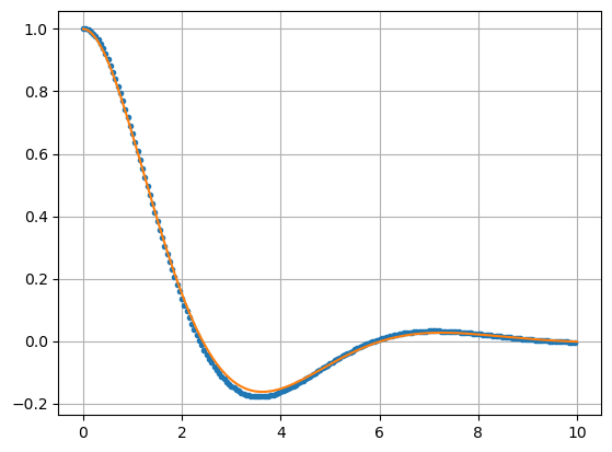
Use odeEulerSys to approximate the solution of the equation

\[ y'' + y + 1 = 0 \ , \ \ y(0)=1 \ , \ \ y'(0) = 0 \]

and compare with the exact solution

\[ y(t) = e^{-t/2} \cos \left( \frac{\sqrt{3}}{2} t \right) + \frac{1}{\sqrt{3}} e^{-t/2} \sin \left( \frac{\sqrt{3}}{2} t \right) \]

a = 1; b = 1; c = 1; tf = 10;

f = lambda t,u: np.array([u[1],(-b*u[1]-c*u[0])/a])
t = np.arange(0,tf,0.05)
u0 = [1,0]
u = odeEulerSys(f,t,u0)
plt.plot(t,u[:,0],'.')

T = np.linspace(0,tf,tf*50)
Y = np.exp(-T/2)*(np.cos(np.sqrt(3)/2*T) + 1/np.sqrt(3)*np.sin(np.sqrt(3)/2*T))
plt.plot(T,Y), plt.grid(True)
plt.show()

See also

Check out Mathematical Python: Systems of Equations for more Python examples using Euler’s method.

Numerical Solutions with SciPy

Euler’s method is simple to understand but it is not accurate enough to use in practice. Higher order Runge-Kutta methods are the standard methods used for real applications but we won’t get into how they work exactly. Instead, let’s just loosely describe a Runge-Kutta method as a “higher order Euler method” and let’s focus on how scipy.integrate.odeint works with systems of differential equations.

The procedure to compute a numerical approximation of a solution of a system of differential equations is:

1. Write the system as a first order system \(\mathbf{u}' = \mathbf{f}(\mathbf{u},t)\), \(\mathbf{u}_0 = \mathbf{u}(t_0)\).

2. Define a Python function f(u,t) for the right hand side \(\mathbf{f}(\mathbf{u},t)\) where parameter u is a vector such that u[k] corresponds to funciton \(u_k(t)\). Note that the variable \(\mathbf{u}\) is first and \(t\) is second.

3. Define vector t of \(t\) values where t[0] is \(t_0\). Usually t = np.linspace(t0,tf,N+1) or equivalently t = np.arange(t0,tf+h,h) where \(h = (t_f - t_0)/N\).

4. Define initial value vector u0 corresponding to \(\mathbf{u}_0 = \mathbf{u}(t_0)\) where \(t_0\) is t[0].

5. Compute the solution u = spi.odeint(f,u0,t). The output of the function is the matrix u of shape (len(t),len(u0)) such that column u[:,k] corresponds to the values of the function \(u_k(t)\) from \(t_0\) to \(t_f\), and row u[n,:] corresponds to the vector \(\mathbf{u}(t_n) = (u_0(t_n),\dots,u_{d-1}(t_n))\) at time \(t_n\).

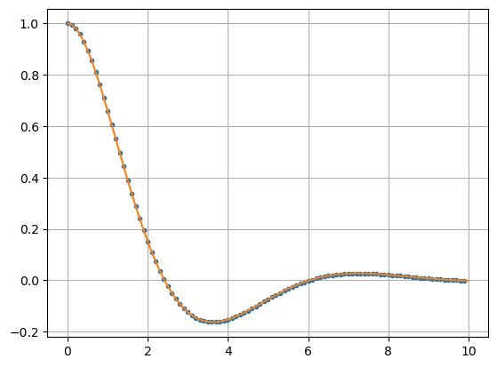
For example, let’s approximate the solution of the equation

\[ y'' + y + 1 = 0 \ , \ \ y(0)=1 \ , \ \ y'(0) = 0 \]

and compare with the exact solution

\[ y(t) = e^{-t/2} \cos \left( \frac{\sqrt{3}}{2} t \right) + \frac{1}{\sqrt{3}} e^{-t/2} \sin \left( \frac{\sqrt{3}}{2} t \right) \]

a = 1; b = 1; c = 1; tf = 10;

f = lambda u,t: np.array([u[1],(-b*u[1]-c*u[0])/a])
t = np.arange(0,tf,0.1)
u0 = [1,0]
u = spi.odeint(f,u0,t)
plt.plot(t,u[:,0],'.')

T = np.linspace(0,tf,tf*50)
Y = np.exp(-T/2)*(np.cos(np.sqrt(3)/2*T) + 1/np.sqrt(3)*np.sin(np.sqrt(3)/2*T))
plt.plot(T,Y), plt.grid(True)
plt.show()

See also

Check out Mathematical Python: Systems of Equations for more Python examples, and SciPy documentation for more information about scipy.integrate.odeint.

Linear Stability Analysis

Consider a first order, \(d\)-dimensional autonomous system of differential equations

\[ \frac{d \mathbf{x}}{dt} = \mathbf{f}(\mathbf{x}) \]

A point \(\mathbf{c} \in \mathbb{R}^d\) is a critical point if \(\mathbf{f}(\mathbf{c}) = \mathbf{0}\). A critical point corresponds to an equilibrium solution (also called a steady state solution)

\[ \mathbf{x}(t) = \mathbf{c} \]

A critical point \(\mathbf{c}\) is an attractor if all solutions which start near \(\mathbf{c}\) converge to \(\mathbf{c}\) as \(t \to \infty\). A critical point \(\mathbf{c}\) is a repeller if all solutions which start near \(\mathbf{c}\) diverge from \(\mathbf{c}\) as \(t \to \infty\). A critical point \(\mathbf{c}\) is a unstable if some solutions which start near \(\mathbf{c}\) converge to \(\mathbf{c}\) and some diverge as \(t \to \infty\).

Let \(\mathbf{c}\) be a critical point and let \(\mathbf{J}_{\mathbf{c}}\) be the Jacobian of the system at \(\mathbf{c}\):

\[\begin{split} \mathbf{J}_{\mathbf{c}} = \begin{bmatrix} \frac{\partial f_0}{\partial x_0} & \cdots & \frac{\partial f_0}{\partial x_{d-1}} \\ \vdots & \ddots & \vdots \\ \frac{\partial f_{d-1}}{\partial x_0} & \cdots & \frac{\partial f_{d-1}}{\partial x_{d-1}} \end{bmatrix} _{\mathbf{x} = \mathbf{c}} \end{split}\]

The linearization theorem allows us to classify critical points:

• if \(\mathrm{Re}(\lambda) < 0\) for each eigenvalue \(\lambda\) of \(\mathbf{J}_{\mathbf{c}}\) then \(\mathbf{c}\) is a attractor

• if \(\mathrm{Re}(\lambda) > 0\) for each eigenvalue \(\lambda\) of \(\mathbf{J}_{\mathbf{c}}\) then \(\mathbf{c}\) is a repeller

• if some eigenvalues of \(\mathbf{J}_{\mathbf{c}}\) have positive real part and some have negative real part then \(\mathbf{c}\) is unstable

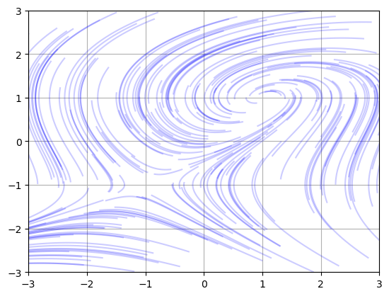
For example, let’s find and classify the critical points of the system

\[\begin{split} \begin{align*} x' &= 1 - y^2 \\ y' &= x - y \end{align*} \end{split}\]

There are 2 critical points: \((1,1)\) and \((-1,-1)\). Compute partial derivatives

\[ \frac{\partial f_1}{\partial x} = 0 \hspace{10mm} \frac{\partial f_1}{\partial y} = -2y \hspace{10mm} \frac{\partial f_2}{\partial x} = 1 \hspace{10mm} \frac{\partial f_2}{\partial y} = -1 \]

Compute eigenvalues of the Jacobians

\[\begin{split} \mathbf{J}_{(1,1)} = \begin{bmatrix} 0 & -2y \\ 1 & -1 \end{bmatrix}_{(1,1)} = \begin{bmatrix} 0 & -2 \\ 1 & -1 \end{bmatrix} \end{split}\]

\[\begin{split} \mathbf{J}_{(-1,-1)} = \begin{bmatrix} 0 & -2y \\ 1 & -1 \end{bmatrix}_{(-1,-1)} = \begin{bmatrix} 0 & 2 \\ 1 & -1 \end{bmatrix} \end{split}\]

J1 = np.array([[0.,-2.],[1.,-1.]])
evals1,evecs1 = la.eig(J1)
print(evals1)

[-0.5+1.32287566j -0.5-1.32287566j]

J2 = np.array([[0.,2.],[1.,-1.]])
evals2,evecs2 = la.eig(J2)
print(evals2)

[ 1.+0.j -2.+0.j]

Therefore \((1,1)\) is an attractor and \((-1,-1)\) is unstable. Let’s plot solutions:

f = lambda u,t: np.array([1 - u[1]**2,u[0] - u[1]])
t = np.linspace(0,1,100)
for _ in range(200):
    u0 = 6*np.random.rand(2) - 3
    u = spi.odeint(f,u0,t)
    plt.plot(u[:,0],u[:,1],c='b',alpha=0.2)
plt.axis([-3,3,-3,3]), plt.grid(True)
plt.show()

See also

Check out Notes on Diffy Qs: Section 8.1 and Section 8.2 for more information and examples about linear classification of critical points.