Scaling

import numpy as np
import scipy.integrate as spi
import matplotlib.pyplot as plt

Simple Example

Consider a simple model of exponential growth where a population \(P\) starts with \(P(0) = P_0\) and increases at a rate proportional to its size. The model is described by the differential equation

\[ \frac{dP}{dt} = rP \ , \ \ P(0) = P_0 \]

for some coefficient \(r\) with dimension T^-1. We can scale the variables \(P\) and \(t\) relative to the parameters \(P_0\) and \(r\) to define new dimensionless parameters \(P^*\) and \(t^*\)

\[ P = P_0 P^* \hspace{10mm} t = \frac{t^*}{r} \]

Make the subsititutions to find the nondimensionalized equation

\[ \frac{dP^*}{dt^*} = P^* \ , \ \ P^*(0) = 1 \]

Therefore the parameters \(P_0\) and \(r\) only affect the scale of the variables in the solution \(P(t)\) and do not change the intrinic behaviour of the system, and so we can study the model without specifying values for \(P_0\) and \(r\). Furthermore, the scaling factors tell us that we should measure population as multiples of the initial value \(P_0\) and time as multiples of \(r^{-1}\).

Nondimensionalization Procedure

The goals of nondimensionalization are:

1. To simplify a mathematical model by reducing the number of parameters in the model.

2. To identify key properties of a mathematical model in terms of dimensionless variables and parameters.

Nondimensionalization is all about choosing a scaling factor \([x]\) (also called charactersitic unit) for each variable \(x\). The nondimensionalization procedure is:

1. Identify all the independent and dependent variables.

2. Replace each variable \(x\) with a quantity \(x = [x]x^*\) where \([x]\) is a scaling factor to be determined and \(x^*\) is dimensionless.

3. Divide all equations in the model by the coefficient of the highest order polynomial or derivative term.

4. Choose the scaling factor for each variable so that the coefficients of as many terms as possible become 1.

5. Rewrite the system of equations in terms of their new dimensionless quantities.

In the previous example, we let \(P = [P]P^*\) and \(t = [t]t^*\) and found

\[ [P] = P_0 \hspace{20mm} [t] = \frac{1}{r} \]

Scaling Conventions

There is usually more than one way to nondimensinalize an equation therefore we need to use our judgement and communicate clearly the choices we make. Here are a few general rules to guide our choices:

1. Scale variables to first simplify equations and then choose scaling factors to simplify initial conditions.

2. Choose the same scaling factor for spatial variables if there is no reason to treat different directions differently.

Scaling Derivatives

Let’s take a closer look at how differential equations transform with scaling. Let \(t\) be the independent variable and let \(x\) be a dependent variable. Introduce scaling factors \([x]\) and \([t]\) and dimensionless variables \(x^*\) and \(t^*\) where

\[ x = [x] x^* \ \ \ \text{and} \ \ \ t = [t] t^* \]

Take the derivative of the equation \(x = [x] t^*\) with respect to \(t\) and use the chain rule to find

\[ \frac{dx}{dt} = [x] \frac{dx^*}{dt} = [x] \frac{dx^*}{dt^*} \frac{dt^*}{dt} = [x] \frac{dx^*}{dt^*} \left( \frac{1}{[t]} \right) = \frac{[x]}{[t]} \frac{dx^*}{dt^*} \]

In general, we have the following rule for derivatives when making substitutions for \(x\) and \(t\):

\[ \frac{d^n x}{dt^n} = \frac{[x]}{[t]^n} \frac{d^n x^*}{dt^{*n}} \]

Mass Spring Equation

Apply the nondimensionalization process to the mass-spring equation:

\[ m \frac{d^2x}{dt^2} + k x = 0 \ , \ \ x(0) = x_0 \ , \ \ \frac{dx}{dt}(0) = 0 \]

Step 1: The independent variable is time \(t\) and the dependent variable is position \(x\).

Step 2: Let \(t = [t] t^*\) and \(x = [x] x^*\). The symbols \([t]\) and \([x]\) are scaling factors to be determined with dimensions T and L respectively. Substitute the new dimensionless variables \(t^*\) and \(x^*\) into the equation:

\[ m \frac{[x]}{[t]^2} \frac{d^2 x^*}{dt^{* 2}} + k [x] x^* = 0 \ , \ \ [x] x^*(0) = x_0 \ , \ \ \frac{[x]}{[t]} \frac{dx^*}{dt^*}(0) = 0 \]

Step 3: Divide the differential equation by the coefficient in the second derivative term and simply rearrange the initial conditions:

\[ \frac{d^2 x^*}{dt^{* 2}} + \frac{k [t]^2}{m} x^* = 0\ , \ \ x^*(0) = \frac{x_0}{[x]} \ , \ \ \frac{dx^*}{dt^*}(0) = 0 \]

Step 4: Choose values for scaling factors \([t]\) and \([x]\) to make coefficients equal to 1:

\[ [t] = \sqrt{ \frac{m}{k} } \hspace{10mm} [x] = x_0 \]

Step 5: Rewrite the system:

\[ \frac{d^2 x^*}{dt^{* 2}} + x^* = 0 \ , \ \ x^*(0) = 1 \ , \ \ \frac{dx^*}{dt^*}(0) = 0 \]

Interpretation: The general solution of the system is

\[ x^*(t^*) = \cos(t^*) \ \ \Rightarrow \ \ x(t) = x_0 \cos( \omega_0 t) \]

where \(\omega_0 = \sqrt{k/m} = 1/[t]\) is the natural frequency and the initial value \(x_0\) is the amplitude of the system. There are no parameters remaining in the nondimensionalized equation therefore the parameters \(m\), \(k\) and \(x_0\) do not change the behaviour of the system but simply change the scale of the variables \(x\) and \(t\).

Logistic Equation

The logistic equation models the growth of a population \(P\) at rate \(r\) limited by a capacity \(K\):

\[ \frac{dP}{dt} = rP(1 - P/K) \ \ , \ \ P(0) = P_0 \]

The dimensions of the left hand side of the equation are N T^-1 since \(P\) is an amount changing over time. For the equation to be dimensionally homogeneous, the parameters \(r\) and \(K\) must have dimensions T^-1 and N respectively. Apply the nondimensionalization process to the logistic equation.

Step 1: Time \(t\) is the independent variable and population \(P\) is the dependent variable.

Step 2: Let \(t = [t] t^*\) and \(P = [P] P^*\) and make the substitution:

\[ \frac{[P]}{[t]} \frac{dP^*}{dt^*} = r[P]P^* - \frac{r[P]^2}{K} (P^*)^2 \ \ , \ \ [P]P^*(0) = P_0 \]

Step 3: Divide by the coefficient of \((P^*)^2\):

\[ \frac{K}{r[P][t]} \frac{dP^*}{dt^*} = \frac{K}{[P]} P^* - (P^*)^2 \ \ , \ \ P^*(0) = \frac{P_0}{[P]} \]

Step 4: Choose scaling factors such that

\[ \frac{K}{r[P][t]} = 1 \ , \ \frac{K}{[P]} = 1 \]

Solve to find \([P] = K\) and \([t] = r^{-1}\).

Step 5: Rewrite the equation:

\[ \frac{dP^*}{dt^*} = P^*(1 - P^*) \ \ , \ \ P^*(0) = \kappa \]

where the initial condition \(\kappa = \frac{P_0}{K}\) describes \(P_0\) as multiples of \(K\).

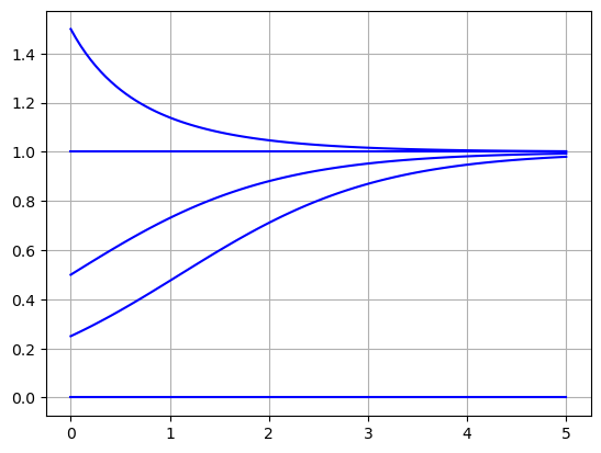
Interpretation: The dimensionless variable \(P^*\) is measured in multiples of the capacity \(K\), and the dimensionless variable \(t^*\) is measured in multiples of \(r^{-1}\).

f = lambda P,t: P*(1 - P)
t = np.linspace(0,5,100)
for P0K in [0.,0.25,0.5,1.,1.5]:
    P = spi.odeint(f,P0K,t)
    plt.plot(t,P,'b')
plt.grid(True)
plt.show()

Lotka-Volterra Equations

The Lotka-Volterra equations model the population dynamics of a predator-prey system:

\[\begin{split} \begin{align*} \frac{dx}{dt} &= \alpha x - \beta xy \\ \frac{dy}{dt} &= \delta xy - \gamma y \end{align*} \end{split}\]

where \(x\) is the population of prey, \(y\) is the population of predators and \(\alpha,\beta,\gamma,\delta\) are parameters. The dimensions of the variables \(x\) and \(y\) are N, the dimensions of the parameters \(\alpha\) and \(\gamma\) are T^-1, and the dimensions of the parameters \(\beta\) and \(\delta\) are N^-1 T^-1. Apply the nondimensionalization process to the Lotka-Volterra equations.

Step 1: Time \(t\) is the independent variable and populations \(x\) and \(y\) are the dependent variables.

Step 2: Let \(t = [t] t^*\), \(x = [x] x^*\), \(y = [y] y^*\) and make the substitutions:

\[\begin{split} \begin{align*} \frac{[x]}{[t]} \frac{dx^*}{dt^*} &= \alpha [x] x^* - \beta [x] [y] x^* y^* \\ \frac{[y]}{[t]} \frac{dy^*}{dt^*} &= \delta [x][y] x^* y^* - \gamma [y]y^* \end{align*} \end{split}\]

Step 3: Divide each equation by the coefficient of \(x^* y^*\):

\[\begin{split} \begin{align*} \frac{1}{\beta [y] [t]} \frac{dx^*}{dt^*} &= \frac{\alpha}{\beta [y]} x^* - x^* y^* \\ \frac{1}{\delta [x] [t]} \frac{dy^*}{dt^*} &= x^* y^* - \frac{\gamma}{\delta [x]}y^* \end{align*} \end{split}\]

Step 4: We see that we should choose

\[ [x] = \frac{\gamma}{\delta} \ \ , \ \ [y] = \frac{\alpha}{\beta} \]

However it is not possible to choose \([t]\) such that all the coefficients are 1. We have two choices:

\[ [t] = \frac{1}{\alpha} \ \ \text{or} \ \ [t] = \frac{1}{\beta} \]

and so we choose (arbitrarily) \([t] = \alpha^{-1}\).

Step 5: Rewrite the system:

\[\begin{split} \begin{align*} \frac{dx^*}{dt^*} &= x^* - x^* y^* \\ \frac{dy^*}{dt^*} &= c \left( x^* y^* - y^* \right) \end{align*} \end{split}\]

where \(c = \frac{\gamma}{\alpha}\).

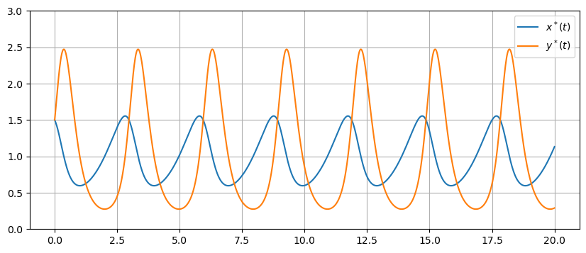
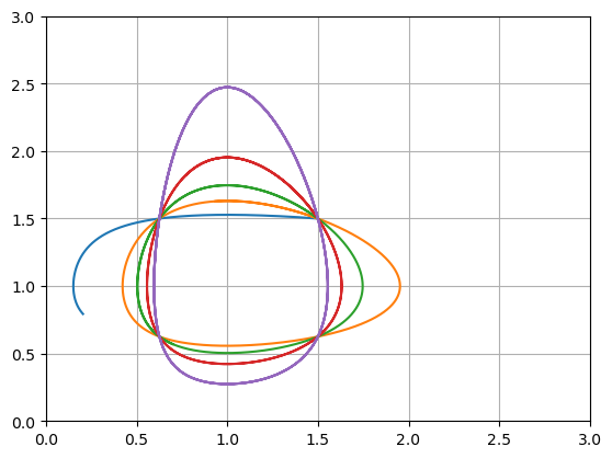
Interpretation: The parameter \(c\) controls how fast \(x^*\) and \(y^*\) change relative to each other. Plot the system for different values of \(c\) to observe the behaviour.

u0 = [1.5,1.5]
t = np.linspace(0,10,1000)
for c in [0.1,0.5,1,2,5]:
    f = lambda u,t: np.array([u[0] - u[0]*u[1],c*(u[0]*u[1] - u[1])])
    U = spi.odeint(f,u0,t)
    plt.plot(U[:,0],U[:,1])
plt.grid(True), plt.xlim([0,3]), plt.ylim([0,3])
plt.show()

u0 = [1.5,1.5]
t = np.linspace(0,20,1000)
c = 5
f = lambda u,t: np.array([u[0] - u[0]*u[1],c*(u[0]*u[1] - u[1])])
U = spi.odeint(f,u0,t)
plt.figure(figsize=(10,4))
plt.plot(t,U[:,0],t,U[:,1])
plt.ylim([0,3]), plt.grid(True), plt.legend(['$x^*(t)$','$y^*(t)$'])
plt.show()