Projectile Motion with Drag

import numpy as np
import scipy.integrate as spi
import matplotlib.pyplot as plt

Problem Statement

Construct a mathematical model of an object shot into the air and subject to the forces of drag and gravity.

Variables and Parameters

Description	Symbol	Dimensions	Type
position of projectile in \(x\)-direction	\(x\)	L	dependent variable
position of projectile in \(y\)-direction	\(y\)	L	dependent variable
time	\(t\)	T	independent variable
mass of the projectile	\(m\)	M	parameter
drag coefficient	\(c\)	MT-1	parameter
constant of gravity	\(g\)	LT-2	parameter
initial velocity	\(v_0\)	LT-1	parameter
initial angle of velocity	\(\theta\)	1	parameter

Assumptions and Constraints

• projectile moves in \(xy\)-plane only

• initial position is at the origin \((0,0)\)

Construction

The force of drag is proportional to velocity and acts in the direction oppposite the velocity

\[ \mathbf{F}_d = -c \| \mathbf{x}'(t) \| \frac{\mathbf{x}'(t)}{\| \mathbf{x}'(t) \|} = -c\left( x',y' \right) \]

The force of gravity acts in the veritcal direction

\[ \mathbf{F}_g = (0,-mg) \]

Apply Newton’s second law to find the equations

\[\begin{split} \begin{align*} m x'' &= - cx' \\ m y'' &= - mg - cy' \\ x(0) &= y(0) = 0 \\ x'(0) &= v_0 \cos \theta \\ y'(0) &= v_0 \sin \theta \end{align*} \end{split}\]

Apply the nondimensionalization procedure. Let \(t = [t]t^*\), \(x = [x]x^*\) and \(y = [y]y^*\) and make the subsitution

\[\begin{split} \begin{align*} \frac{m[x]}{[t]^2} \frac{d^2x^*}{dt^{*2}} &= -\frac{c[x]}{[t]} \frac{dx^*}{dt^*} \\ \frac{m[y]}{[t]^2} \frac{d^2y^*}{dt^{*2}} &= -mg - \frac{c[y]}{[t]} \frac{dy^*}{dt^*} \\ x^*(0) &= y^*(0) = 0 \\ \frac{[x]}{[t]} \frac{dx^*}{dt^*}(0) &= v_0 \cos \theta \\ \frac{[y]}{[t]} \frac{dy^*}{dt^*}(0) &= v_0 \sin \theta \end{align*} \end{split}\]

Divide by second derivative term and simplify

\[\begin{split} \begin{align*} \frac{d^2x^*}{dt^{*2}} &= -\frac{c[t]}{m} \frac{dx^*}{dt^*} \\ \frac{d^2y^*}{dt^{*2}} &= -\frac{g[t]^2}{[y]} - \frac{c[t]}{m} \frac{dy^*}{dt^*} \\ x^*(0) &= y^*(0) = 0 \\ \frac{dx^*}{dt^*}(0) &= v_0 \frac{[t]}{[x]} \cos \theta \\ \frac{dy^*}{dt^*}(0) &= v_0 \frac{[t]}{[y]} \sin \theta \end{align*} \end{split}\]

Choose \([t] = \frac{m}{c}\) and \([x] = [y] = \frac{gm^2}{c^2}\) and write

\[\begin{split} \begin{align*} \frac{d^2x^*}{dt^{*2}} &= -\frac{dx^*}{dt^*} \\ \frac{d^2y^*}{dt^{*2}} &= -1 - \frac{dy^*}{dt^*} \\ x^*(0) &= y^*(0) = 0 \\ \frac{dx^*}{dt^*}(0) &= v^*_0 \cos \theta \\ \frac{dy^*}{dt^*}(0) &= v^*_0 \sin \theta \end{align*} \end{split}\]

where \(v_0^* = \frac{v_0c}{gm}\). These equations are independent of each other and can be solved analytically. However, we will approximate solutions using SciPy using the first order system with \(u_0 = x^*\), \(u_1 = \frac{dx^*}{dt^*}\), \(u_2 = y^*\), \(u_3 = \frac{dy^*}{dt^*}\):

\[\begin{split} \begin{align*} \frac{du_0}{dt^*} &= u_1 \\ \frac{du_1}{dt^*} &= -u_1 \\ \frac{du_2}{dt^*} &= u_3 \\ \frac{du_3}{dt^*} &= - 1 - u_3 \\ u_0(0) &= u_2(0) = 0 \\ u_1(0) &= v^*_0 \cos \theta \\ u_3(0) &= v^*_0 \sin \theta \end{align*} \end{split}\]

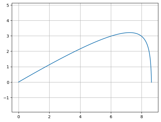
Analysis

def f(u,t):
    dudt = np.zeros(4)
    dudt[0] = u[1]
    dudt[1] = -u[1]
    dudt[2] = u[3]
    dudt[3] = -1 - u[3]
    return dudt

v0 = 10; theta = np.pi/6
u0 = [0,v0*np.cos(theta),0,v0*np.sin(theta)]
t = np.linspace(0,6,200)
u = spi.odeint(f,u0,t)
plt.plot(u[:,0],u[:,2]), plt.axis('equal'), plt.grid(True)
plt.show()