Simple Pendulum

import numpy as np
import matplotlib.pyplot as plt
import scipy.integrate as spi

Problem Statement

A pendulum is a mass attached to one end of a rod which is fixed at the other end and swings about the fixed end under the force of gravity. How does the pendulum swing over time based on initial position and velocity?

Variables and Parameters

Description	Symbol	Dimensions	Type
angle of the pendulum	\(\theta\)	1	dependent variable
time	\(t\)	T	independent variable
length of rod	\(L\)	L	parameter
mass of the object	\(m\)	M	parameter
constant of gravity	\(g\)	LT-2	parameter
initial angular position	\(\theta_0\)	1	parameter
initial angular velocity	\(\omega_0\)	T-1	parameter

Constraints and Assumptions

• no drag, damping or friction

• mass is a point

• rod has no mass and no drag

Construction

The position of the mass is given by the angle \(\theta\):

\[\begin{split} \begin{align*} x &= L \sin \theta \\ y &= -L \cos \theta \end{align*} \end{split}\]

Let \(F\) be the magnitude of the force in the rod acting on the mass. Since \(F\) acts in the direction of the rod from the mass to the origin we have

\[ \mathbf{F} = \left( - F \sin \theta , F \cos \theta \right) \]

Apply Newton’s second law

\[\begin{split} \begin{align*} m x'' &= -F \sin \theta \\ m y'' &= F \cos \theta - mg \end{align*} \end{split}\]

We don’t have an expression for \(F\) and so we want to combine the equations above to eliminate the variable \(F\). Since \(x = L \sin \theta \) and \(y = - L \cos \theta\) and \(L\) is constant we have

\[\begin{split} \begin{align*} x' &= \theta' L \cos \theta \\ x'' &= - (\theta')^2 L \sin \theta + \theta'' L \cos \theta \\ y' &= \theta' L \sin \theta \\ y'' &= (\theta')^2 L \cos \theta + \theta'' L \sin \theta \end{align*} \end{split}\]

therefore we can rewrite the system of equations in terms of \(\theta\):

\[\begin{split} \begin{align*} m (- (\theta')^2 L \sin \theta + \theta'' L \cos \theta) &= -F\sin \theta \\ m ((\theta')^2 L \cos \theta + \theta'' L \sin \theta) &= F \cos \theta - mg \end{align*} \end{split}\]

Multiply the first equation by \(\cos \theta\) and the second equation by \(\sin \theta\) and add to get

\[ m L \theta'' = - mg \sin \theta \]

and finally

\[ \theta'' + \frac{g}{L} \sin \theta = 0 \ , \ \ \theta(0) = \theta_0 \ , \ \ \theta'(0) = \omega_0 \]

Apply the nondimensionalization procedure. Let \(\theta = [\theta] \theta^*\) and \(t = [t] t^*\) and write

\[ \frac{[\theta]}{[t]^2} \frac{d^2 \theta^*}{dt^{*2}} + \frac{g}{L} \sin([\theta] \theta^*) = 0 \ , \ \ [\theta]\theta^*(0) = \theta_0 \ , \ \ \frac{[\theta]}{[t]} \frac{d\theta^*}{dt^*}(0) = \omega_0 \]

Divide by the second order term and simplify

\[ \frac{d^2 \theta^*}{dt^{*2}} + \frac{g [t]^2}{L [\theta]} \sin([\theta] \theta^*) = 0 \ , \ \ \theta^*(0) = \frac{\theta_0}{[\theta]} \ , \ \ \frac{d\theta^*}{dt^*}(0) = \omega_0 \frac{[t]}{[\theta]} \]

There are several choices and we choose \([\theta] = 1\) and \([t] = \sqrt{\frac{L}{g}}\) and we arrive at the equation

\[ \frac{d^2 \theta}{dt^{*2}} + \sin \theta = 0 \ , \ \ \theta(0) = \theta_0 \ , \ \ \frac{d\theta}{dt^*}(0) = \omega_0 \sqrt{\frac{L}{g}} \]

Introduce new variables \(u_0 = \theta\) and \(u_1 = \frac{d\theta}{dt^*}\) and write

\[\begin{split} \begin{align*} \frac{d u_0}{dt^*} &= u_1 \\ \frac{d u_1}{dt^*} &= -\sin u_0 \end{align*} \end{split}\]

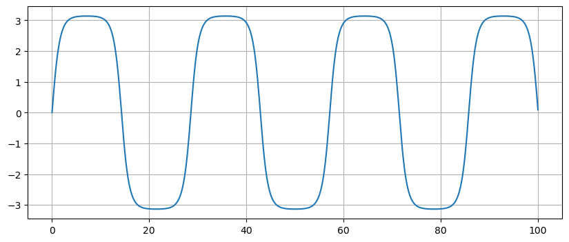
Plot solutions for different initial conditions:

f = lambda u,t: np.array([u[1],-np.sin(u[0])])
u0 = [0.,1.99999]
t = np.linspace(0,100,1000)
u = spi.odeint(f,u0,t)

plt.figure(figsize=(10,4))
plt.plot(t,u[:,0]), plt.grid(True)
plt.show()

Analysis

Under construction