Laws of Motion and Forces

import numpy as np
import scipy.integrate as spi
import matplotlib.pyplot as plt

Newton’s Second Law of Motion

Newton’s second law of motion states that the change in an object’s momentum is proprotional to the force acting on it. In other words, if an object has mass \(m\) and position \(\mathbf{p}(t) = (x(t),y(t),z(t))\) then

\[ m \frac{d^2 \mathbf{p}}{dt^2} = \mathbf{F} \]

where the right hand side is the total sum of forces acting on the object. Let \(\mathbf{F} = (F_x,F_y,F_z)\) be the components of the force vector and write Newton’s second law as a second order, 3-dimensional system of differential equations:

\[\begin{split} \begin{align*} \frac{d^2x}{dt^2} &= \frac{F_x}{m} \\ \frac{d^2y}{dt^2} &= \frac{F_y}{m} \\ \frac{d^2z}{dt^2} &= \frac{F_z}{m} \end{align*} \end{split}\]

Therefore we can construct a deterministic mathematical model of an object in motion by applying constitutive laws to model the forces in a system. Each constitutive law below is itself a mathematical model and has its own assumptions and constraints built in.

See also

Check out Wikipedia: Newton’s Laws of Motion for more information.

Newton’s Law of Gravity

Newton’s law of gravity states that an object attracts another object with a force that is proportional to the product of their masses and inversely proportional to the square of the distance between their centers. Therefore if the first object has mass \(m_1\) and position \(\mathbf{p}_1\), and the second object has mass \(m_2\) and position \(\mathbf{p}_2\) then the force acting on the second object is

\[ \mathbf{F}_g = \frac{G m_1 m_2}{\| \mathbf{p}_1 - \mathbf{p}_2 \|^2} \left( \mathbf{p}_1 - \mathbf{p}_2 \right) \]

where \(G\) is the graviational constant with dimensions L³T^-2M^-1. The gravitational force exerted by the Earth on an object of mass \(m\) on the surface of the Earth is

\[ F_g = m g \]

where \(g = GM/R^2\) has dimensions LT^-2, and \(M\) and \(R\) are the mass and radius of the Earth.

See also

Check out Wikipedia: Newton’s Law of Universal Graviation and Wikipedia: Gravity of Earth for more information.

Spring Force

Hooke’s law states that the force required to stretch/compress a spring by a distance \(x\) is proportional to \(x\). in other words, the spring force is

\[ F_s = kx \]

for a spring constant \(k\) with dimensions MT^-2.

See also

Check out Wikipedia: Hooke’s Law for more information.

Drag and Damping Forces

Stokes’ law states that the force exerted on an object moving through a fluid is proportional to the speed of the object. In other words, the drag force equation is

\[ F_d = c v \]

where \(v\) is the speed of the object and \(c\) is the drag coefficient with units MT^-1.

A damper is a device that uses fluid to exert force on a moving object. Shock absorbers in bikes and cars are examples of dampers. The damping force equation is the same as the drag equation but we call \(c\) the damping coefficent.

Note that drag and damping forces always act in the direction opposite to the motion of the object.

See also

Check out Wikipedia: Stokes law and Wikipedia: Dashpot for more information.

Examples

Mass Spring Damper System in 1D

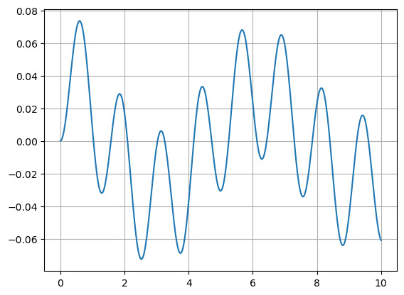
Consider a mass sliding in the \(x\)-direction on a frictionless surface attached to a spring and damper and subject to a time-dependent external force \(F(t)\). Applying Newton’s second law yields the equation

\[ m x'' = -cx' - kx + F(t) \]

where the right hand side is the sum of forces acting in the \(x\)-direction. Rearranging gives the equation of motion of a mass attached to a spring and damper with an applied external force is

\[ m x'' + cx' + kx = F(t) \]

Let’s plot the solution for a sinusoidal forcing function \(F(t) = \cos(\omega t)\).

t = np.linspace(0,10,500)
m = 1; c = 0.1; k = 1; w = 5;
F = lambda t: np.cos(w*t)
f = lambda u,t: np.array([u[1],(F(t) - c*u[1] - k*u[0])/m])
u0 = [0,0]
u = spi.odeint(f,u0,t)

plt.plot(t,u[:,0]), plt.grid(True)
plt.show()

See also

Check out Notes on Diffy Qs: Section 2.4 and Section 2.6 for more about mechanical vibrations.