Kernel Density Estimation

import numpy as np
import matplotlib.pyplot as plt
from scipy import stats

What is Density Estimation?

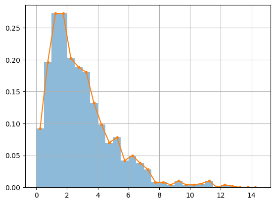
Suppose we have a method of computing or observing random samples of a continuous random variable \(X\) however we do not know its probability distribution function \(f(x)\). The goal of density estimation is to approximate \(f(x)\) using a collection random samples of \(X\). The simplest kind of density estimation is simply to plot the histogram of the samples.

For example, let \(X_1 \sim Exp(\lambda_1)\) and \(X_2 \sim Exp(\lambda_2)\) and let \(Y = X_1 + X_2\). Compute random samples and plot the histogram.

N = 1000
X1 = stats.expon.rvs(scale=1,size=N)
X2 = stats.expon.rvs(scale=2,size=N)
Y = X1 + X2
freqs,bins,_ = plt.hist(Y,bins=np.arange(0,15,0.5),density=True,alpha=0.5)
mids = (bins[:-1] + bins[1:])/2
plt.plot(mids,freqs,'.-')
plt.grid(True)
plt.show()

See also

Check out Wikipedia: Kernel Density Estimation for more information.

Kernel Functions

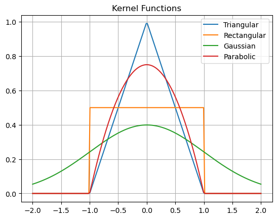
A kernel is a function \(K : \mathbb{R} \rightarrow \mathbb{R}\) such that \(K(x) \ge 0\) and \(K(x) = K(-x)\) for all \(x \in \mathbb{R}\), and \(\int_{-\infty}^{\infty} K(x) \, dx = 1\). In other words, a kernel function is a symmetric probability density function. For example:

The triangular kernel function is

\[\begin{split} K(x) = \left\{ \begin{array}{ccc} 1-|x| & , & |x| \le 1 \\ 0 & , & x > 1 \end{array} \right. \end{split}\]

The rectangular kernel function is

\[\begin{split} K(x) = \left\{ \begin{array}{ccc} 1/2 & , & |x| \le 1 \\ 0 & , & x > 1 \end{array} \right. \end{split}\]

The gaussian kernel function is

\[ K(x) = \frac{1}{\sqrt{2\pi}} e^{-x^2/2} \]

The parabolic kernel function is

\[\begin{split} K(x) = \left\{ \begin{array}{ccc} \frac{3}{4}(1 - x^2) & , & |x| \le 1 \\ 0 & , & x > 1 \end{array} \right. \end{split}\]

# u(x) = 1 if |x| < 1
u = lambda x: np.heaviside(x + 1,1) - np.heaviside(x - 1,1)

x = np.linspace(-2,2,200)
K1 = (1 - np.abs(x))*u(x)
K2 = 0.5*u(x)
K3 = 1/np.sqrt(2*np.pi)*np.exp(-x**2/2)
K4 = 0.75*(1 - x**2)*u(x)

plt.plot(x,K1,label = 'Triangular')
plt.plot(x,K2,label = 'Rectangular')
plt.plot(x,K3,label = 'Gaussian')
plt.plot(x,K4,label = 'Parabolic')
plt.title('Kernel Functions'), plt.legend(), plt.grid(True)
plt.show()

Kernel Density Functions

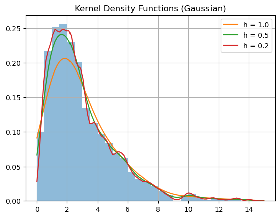
Let \(x_1,\dots,x_N\) be samples of a random variable \(X\) with unknown probability density function \(f(x)\). Choose a kernel \(K(x)\) and bandwidth parameter \(h>0\) and define the kernel density function

\[ \hat{f}_h(x) = \frac{1}{Nh} \sum \limits_{i=1}^N K \left( \frac{x - x_i}{h} \right) \]

The function \(\hat{f}_h(x)\) is a probabilty density function and is an estimate of \(f(x)\). Optimal values of \(h\) are determined by methods beyond the scope of this course. However we just recognize that increasing \(h\) provides a smoother result but loses some of the shape of the data.

Let’s constuct kernel density functions for the example above.

N = 1000
X1 = stats.expon.rvs(scale=1,size=N)
X2 = stats.expon.rvs(scale=2,size=N)
Y = X1 + X2

plt.hist(Y,bins=np.arange(0,15,0.5),density=True,alpha=0.5)
K = lambda x: 1/np.sqrt(2*np.pi)*np.exp(-x**2/2)
fh = lambda x,h: 1/(len(Y)*h)*sum([K((x - Y[i])/h) for i in range(len(Y))])
x = np.linspace(0,15,100)
plt.plot(x,fh(x,1),label='h = 1.0')
plt.plot(x,fh(x,0.5),label='h = 0.5')
plt.plot(x,fh(x,0.2),label='h = 0.2')
plt.title('Kernel Density Functions (Gaussian)'), plt.legend(), plt.grid(True)
plt.show()

plt.hist(Y,bins=np.arange(0,15,0.5),density=True,alpha=0.5)
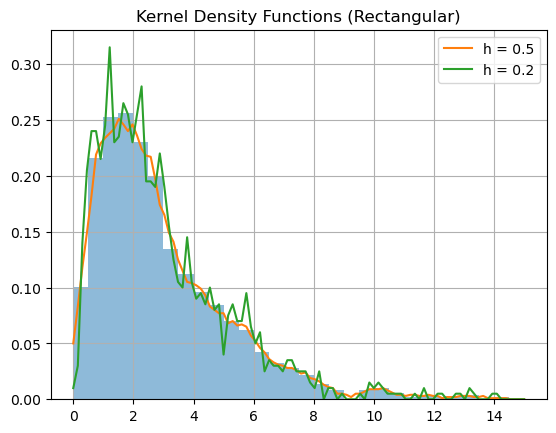
K = lambda x: 0.5*u(x)
fh = lambda x,h: 1/(len(Y)*h)*sum([K((x - Y[i])/h) for i in range(len(Y))])
x = np.linspace(0,15,100)
plt.plot(x,fh(x,0.5),label='h = 0.5')
plt.plot(x,fh(x,0.1),label='h = 0.2')
plt.title('Kernel Density Functions (Rectangular)'), plt.legend(), plt.grid(True)
plt.show()

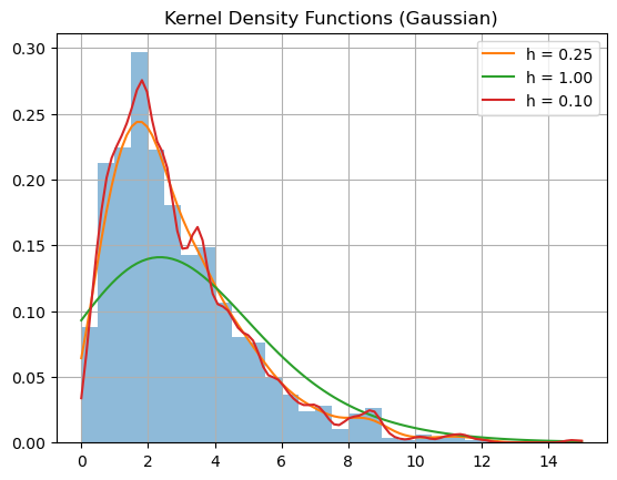
KDE with SciPy

The function scipy.stats.gaussian_kde computes the kernel density function with the gaussian kernel. It automatically computes the optimal bandwidth parameter. We can also specify the bandwidth by setting the value of the bw_method parameter. Let’s again compute kernel density functions for the example above.

N = 1000
X1 = stats.expon.rvs(scale=1,size=N)
X2 = stats.expon.rvs(scale=2,size=N)
Y = X1 + X2

plt.hist(Y,bins=np.arange(0,15,0.5),density=True,alpha=0.5)
kde1 = stats.gaussian_kde(Y)
kde2 = stats.gaussian_kde(Y,bw_method=1)
kde3 = stats.gaussian_kde(Y,bw_method=0.1)

x = np.linspace(0,15,100)
plt.plot(x,kde1(x),label='h = {:.2f}'.format(kde1.factor))
plt.plot(x,kde2(x),label='h = 1.00')
plt.plot(x,kde3(x),label='h = 0.10')
plt.title('Kernel Density Functions (Gaussian)'), plt.legend(), plt.grid(True)
plt.show()

See also

Check out the SciPy tutorial on kernel density estimation.