Linear Regression

import numpy as np
import matplotlib.pyplot as plt
import scipy.linalg as la
import pandas as pd

Linear Regression

A linear regression model is a function of the form

\[ f(\mathbf{x} ; \boldsymbol{\beta}) = \beta_0 + \beta_1 x_1 + \beta_2 x_2 + \dots + \beta_p x_p \]

where \(\mathbf{x} = (x_1,\dots,x_p)\) and \(\boldsymbol{\beta} = (\beta_0,\beta_1,\dots,\beta_p)\).

Least Squares

Least squares regression corresponds to the case where we choose the sum of squared errors cost function

\[ C = \sum_{i=0}^N |y_i - f(\mathbf{x}_i ; \boldsymbol{\beta} ) |^2 \]

For simple linear regression this corresponds to

\[ C = || \mathbf{y} - X \boldsymbol{\beta} ||^2 \]

where

\[\begin{split} \mathbf{y} = \begin{bmatrix} y_0 \\ y_1 \\ \vdots \\ y_N \end{bmatrix} \hspace{20mm} X = \begin{bmatrix} 1 & x_0 \\ 1 & x_1 \\ \vdots & \vdots \\ 1 & x_N \end{bmatrix} \hspace{20mm} \boldsymbol{\beta} = \begin{bmatrix} \beta_0 \\ \beta_1 \end{bmatrix} \end{split}\]

Note that \(X \boldsymbol{\beta}\) is a vector in the column space of \(X\) therefore the distance \(|| \mathbf{y} - X \boldsymbol{\beta} ||\) is minimized when the line from \(\mathbf{y}\) to \(X\boldsymbol{\beta}\) is orthogonal to the column space. In other words, we want to find \(\boldsymbol{\beta}\) such that \(X^T(\mathbf{y} - X \boldsymbol{\beta}) = 0\) which leads to the normal equations

\[ X^T X \boldsymbol{\beta} = X^T \mathbf{y} \]

Residuals

The difference between the observed value \(y_i\) and the predicted value \(f(\mathbf{x}_i ; \boldsymbol{\beta})\) is called the residual

\[ \varepsilon_i = y_i - f(\mathbf{x}_i ; \boldsymbol{\beta}) \]

Example: Real Estate Prices

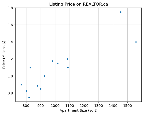
The data below was collected from REALTOR.ca for 2-bedroom apartments for sale in the Kitsilano neighborhood of Vancouver. The dependent variable \(y\) is the listing price and the independent variable \(x\) is the apartment size (in square feet).

x = [1557,1452,767,900,1018,802,924,981,879,819,829,1088,1085]
y = [1.398,1.750,0.899,0.848,1.149,0.825,0.999888,1.175,0.885,0.749888,1.098,1.099,1.198]
plt.plot(x,y,'.')
plt.title('Listing Price on REALTOR.ca')
plt.xlabel('Apartment Size (sqft)'), plt.ylabel('Price (Millons $)'), plt.grid(True)
plt.show()

Choose a simple linear regression model for the data \(y = \beta_0 + \beta_1 x + \varepsilon\). Construct the matrix \(X\):

X = np.column_stack([np.ones(len(x)),x])
X

array([[1.000e+00, 1.557e+03],
       [1.000e+00, 1.452e+03],
       [1.000e+00, 7.670e+02],
       [1.000e+00, 9.000e+02],
       [1.000e+00, 1.018e+03],
       [1.000e+00, 8.020e+02],
       [1.000e+00, 9.240e+02],
       [1.000e+00, 9.810e+02],
       [1.000e+00, 8.790e+02],
       [1.000e+00, 8.190e+02],
       [1.000e+00, 8.290e+02],
       [1.000e+00, 1.088e+03],
       [1.000e+00, 1.085e+03]])

Solve the normal equations:

beta = la.solve(X.T@X,X.T@y)
beta

array([0.10620723, 0.00096886])

Plot the linear regression model with the data:

xs = np.linspace(700,1600)
ys = beta[0] + beta[1]*xs
plt.plot(x,y,'.',xs,ys)
plt.title('Listing Price on REALTOR.ca'), plt.grid(True)
plt.xlabel('Apartment Size (sqft)'), plt.ylabel('Price (Millons $)')
plt.show()

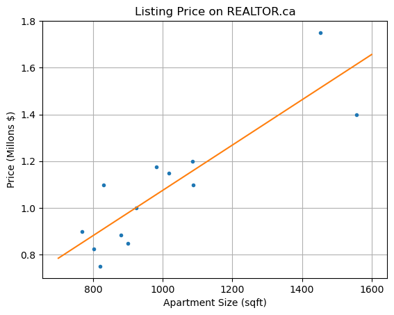
The coefficient \(\beta_1 = 0.00096886\) suggests that the listing price of a 2-bedroom apartment increases by \(968.86\) dollars per square foot.

Example: Temperature

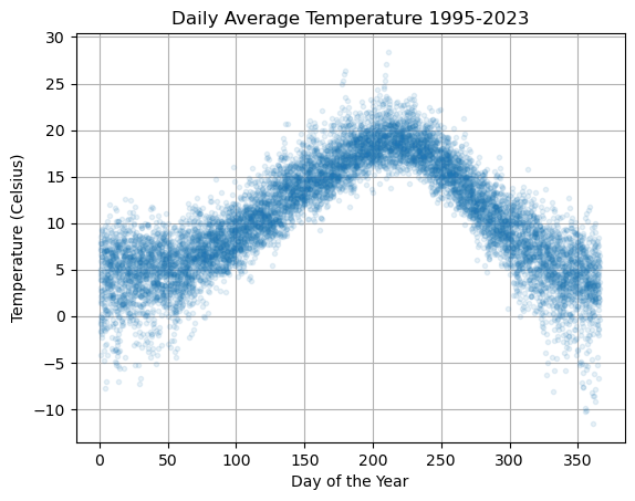
Vancouver weather data is available at vancouver.weatherstats.ca. Plot the daily average temperature as function of the day of the year.

df = pd.read_csv('temperature.csv')

df.head()

	day	month	year	dayofyear	avg_temperature
0	13	4	2023	103	7.10
1	12	4	2023	102	5.19
2	11	4	2023	101	8.00
3	10	4	2023	100	7.69
4	9	4	2023	99	9.30

df.tail()

	day	month	year	dayofyear	avg_temperature
9995	1	12	1995	335	6.40
9996	30	11	1995	334	9.15
9997	29	11	1995	333	11.50
9998	28	11	1995	332	9.75
9999	27	11	1995	331	6.90

plt.plot(df['dayofyear'],df['avg_temperature'],'.',alpha=0.1,lw=0)
plt.title('Daily Average Temperature 1995-2023')
plt.xlabel('Day of the Year'), plt.ylabel('Temperature (Celsius)'), plt.grid(True)
plt.show()

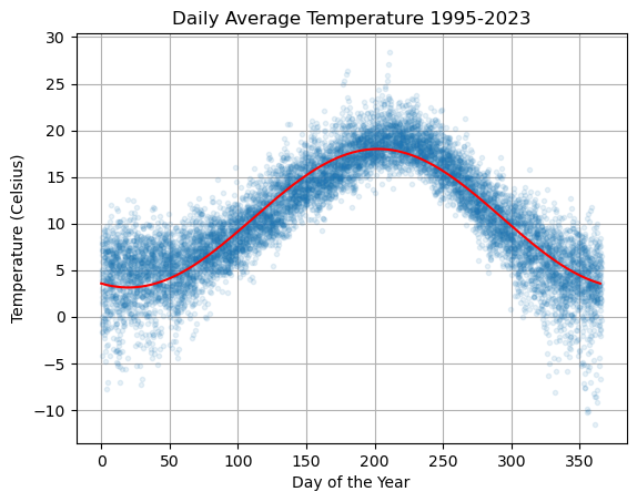
Let \(T\) by the temperature and let \(d\) be the day of the year. Define a regression model of the form

\[ T = \beta_0 + \beta_1 \cos(2 \pi d/365) + \beta_2 \sin(2 \pi d/365) \]

Note that if we rewrite the variables as \(y = T\), \(x_1 = \cos(2 \pi d/365)\) and \(x_2 = \sin(2 \pi d/365)\) then we see that this is indeed a linear regression model

\[ y = \beta_0 + \beta_1 x_1 + \beta_2 x_2 \]

Construct the corresponding data matrix \(X\) and compute the coefficient vector \(\boldsymbol{\beta}\).

N = len(df)
d = df['dayofyear']
T = df['avg_temperature']
X = np.column_stack([np.ones(N),np.cos(2*np.pi*d/365),np.sin(2*np.pi*d/365)])
beta = la.solve(X.T@X,X.T@T)

ds = np.linspace(0,365,500)
Ts = beta[0] + beta[1]*np.cos(2*np.pi*ds/365) + beta[2]*np.sin(2*np.pi*ds/365)

plt.plot(df['dayofyear'],df['avg_temperature'],'.',alpha=0.1,lw=0)
plt.plot(ds,Ts,'r'), plt.grid(True)

plt.title('Daily Average Temperature 1995-2023')
plt.xlabel('Day of the Year'), plt.ylabel('Temperature (Celsius)')
plt.show()

f = lambda d,beta: beta[0] + beta[1]*np.cos(2*np.pi*d/365) + beta[2]*np.sin(2*np.pi*d/365)
residual = T - f(d,beta)
plt.hist(residual,bins=50,density=True)
plt.show()

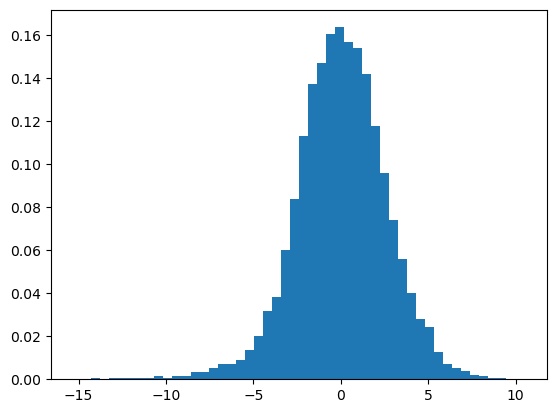
la.norm(residual)/N

0.026025310340052316

Example: Temperature

We can see in teh previous example that the linear model doesn’t quite fit the data. Let’s modify our linear regression model to include periodic functions with periods of 1 year (365 days) and 6 months (365/2 days):

\[ T = \beta_0 + \beta_1 \cos(2 \pi d/365) + \beta_2 \sin(2 \pi d/365) + \beta_3 \cos(4 \pi d/365) + \beta_4 \sin(4 \pi d/365) \]

Construct the corresponding data matrix \(X\) and compute the coefficient vector \(\boldsymbol{\beta}\).

N = len(df)
d = df['dayofyear']
T = df['avg_temperature']
X = np.column_stack([np.ones(N),
                     np.cos(2*np.pi*d/365),np.sin(2*np.pi*d/365),
                     np.cos(4*np.pi*d/365),np.sin(4*np.pi*d/365)])
beta = la.solve(X.T@X,X.T@T)

ds = np.linspace(0,365,500)
x1 = np.cos(2*np.pi*ds/365)
x2 = np.sin(2*np.pi*ds/365)
x3 = np.cos(4*np.pi*ds/365)
x4 = np.sin(4*np.pi*ds/365)
Ts = beta[0] + beta[1]*x1 + beta[2]*x2 + beta[3]*x3 + beta[4]*x4

plt.plot(df['dayofyear'],df['avg_temperature'],'.',alpha=0.1,lw=0)
plt.plot(ds,Ts,'r'), plt.grid(True)
plt.title('Daily Average Temperature 1995-2023')
plt.xlabel('Day of the Year'), plt.ylabel('Temperature (Celsius)')
plt.show()

f = lambda d,beta: beta[0] + beta[1]*np.cos(2*np.pi*d/365) + beta[2]*np.sin(2*np.pi*d/365) + beta[3]*np.cos(4*np.pi*d/365) + beta[4]*np.sin(4*np.pi*d/365)
residual = T - f(d,beta)
plt.hist(residual,bins=50,density=True)
plt.show()

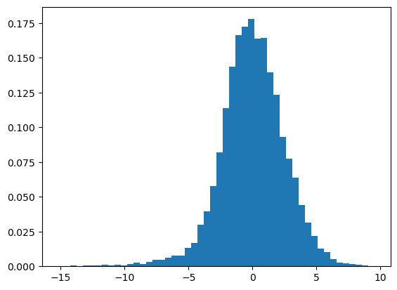
la.norm(residual)/N

0.02490190968939154