Wind Energy#
import numpy as np
import matplotlib.pyplot as plt
from scipy import stats
import pandas as pd
Wind Power Density#
Consider air with density \(\rho\) moving through an area \(A\) at speed \(U\) (in the direction perpendicular to the area \(A\)). The mass flow rate is
and has units M T-1. The kinetic energy of mass \(m\) moving at speed \(U\) is given by
Wind power is the rate of kinetic energy flow of air through the given area and is given by
Wind power generated by a turbine depends on the swept area of the wind turbine blades and so we usually normalize the power by dividing by the area to assess to the wind power density:
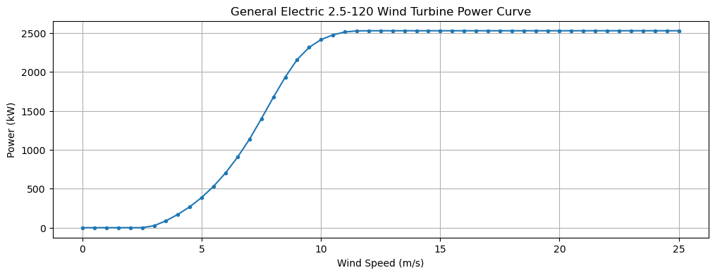
Turbine Power Curve#
A wind turbine only captures a fraction of the total wind power available and a turbine usually operates only within a range of wind speeds from the cut-in wind speed up to the cut-out wind speed. Each turbine has a power curve which specifies the power output as a function of wind speed. The curve is usually an \(S\)-shaped curve from 0kW up to a maximum rated power. For example, the curve below shows data for a General Electric 2.5-200 wind turbine with cut-in speed 3m/s and cut-out speed 25m/s. The data was taken from wind-turbine-models.com.
U = np.arange(0,25.5,0.5)
P = np.hstack([[0,0,0,0,0,0,
                25,89,171,269,389,533,704,906,1136,1400,1674,1934,2160,2316,2416,2477,2514,2528],
                2530*np.ones(27)])
plt.figure(figsize=(12,4))
plt.plot(U,P,'.-'), plt.grid(True)
plt.xlabel('Wind Speed (m/s)'), plt.ylabel('Power (kW)')
plt.title('General Electric 2.5-120 Wind Turbine Power Curve')
plt.show()
See also
Check out wind-turbine-models.com to see design specifications for different kinds of turbines.
Estimating Wind Power Generation#
Consider a wind turbine with a power curve given by a function \(P(U)\) of the wind speed \(U\). Wind speed \(U\) changes over time \(t\) and so the total energy generated from time \(t_0\) to \(t_f\) is given by
If we have wind speed measurements \(U_0,\dots,U_N\) at intervals \(\Delta t = t_{i+1} - t_i\) (where \(U_i\) is wind speed at time \(t_i\)) then the total energy is
Note that the approximation is given by the trapezoid rule.