Probability Distributions#
Learning Goals#
Define random variable, probability distributions, and cumulative distributions
Generate a probability distribution from data
Basic Concepts in Probability#
A random variable is …
The Poisson distribution is
A population is … A sample space is …
For example, all students registered in 3rd year math courses is a population and the subset of students taking math 360 is a sample from that population.
Probability allows us to go from the population to the sample: that is, probability allows us to draw conclusions about the characteristics of a hypothetical subset taken from the population, based on the features of the population. For example, if we know that the average math grade in our population of students taking 3rd year math courses is a B+. We could then suggest that the average math grade of students taking math 360 is a B+.
Statistics allows us to go from the sample to the population: that is, statistics allows us to draw conclusions about the characteristics of the population with (inferential) statistics. For example, if we calculated the average math grade of students in math 360, we could use this value to infer the average math grade of all students registered in 3rd year math courses (there are ways of rigorously showing such an inference, but that is outside the scope of math 360).
Statistics one of the most commonly misused areas of mathematics and is often used to misrepresent data. (Check out the wikipedia article: misuse of statistics).
Terminology#
Some preliminary definitions to get us started:
Experiment: a process that generates a set of data. E.g., flipping a coin. In this experiement, there are two possible outcomes – heads or tails.
Outcome: something that can happen in an experiment. E.g., heads is a possible outcome from flipping a coin.
Event: a collection of outcomes that can be assigned a probability. E.g., flipping a (fair) coin twice, an event is flipping a head on the first flip and a head on the second flip.
Here, by saying fair, we mean that all outcomes are equally likely.
Probability: the likelihood that somthing will happen. E.g., on a fair coin, the probability of heads is 1/2 or 50%. In other words, the likelihood of us flipping a head is about half.
To calculate the probabilty, we first need to find the total number of possible outcomes. For a single coin flip this is 2: either heads or tails. We then need to find the total number of outcomes in the event we are interested in. In the case of flipping a head, there is only one event where this happens, so the probability is then 1/2 =0.5.
Independent: two events are independent if the occurence of one has no impact on the occurance of the other. E.g., when flipping a (fair) coin twice, the outcome of the first flip has no impact on the second flip.
Mean: the average or expected value. In terms of a probability distribution, the mean is the long-term average value of the random variable.
Variability: A measure of spread in the data. Large amounts of variability in experiments “hide” scientific findings.
Variance, \(\sigma^2\): A way to measure variability. A small variance means that the data is tightly clumped together, whereas a large variance means that the data is more spread out.
Standard deviation: Calculated from variance as \(s = \sqrt{\sigma^2}\). The standard deviation shows how spread out the data is from the mean. A small standard deviation means the data is close to the mean, whereas a large standard deviation means the data has a bit of spread away from the mean. The standard deviation is also sometimes written as just \(\sigma\), with the variance then defined as the square of the standard deviation.
Remarks:
the mean, variance, and standard deviation (as well as other measures like median and mode) are often referred to as Descriptive Statistics because they describe the data. These quantities are not typically called parameters, but rather statistics.
we use Inferential Statistics to leverage our knowledge of the sample’s statistics to say something about the entire population (in other words, make an inference).
Probability#
Definition If an experiment can result in any one of \(N\) different equally likely outcomes, and if exactly \(n\) of these outcomes correspond to event \(A\), then the probability of event \(A\) is \(P(A) = \frac{n}{N}\).
Example: Let’s toss a fair coin 2 times. Calculate the probability \(P(A)\) that at least one tail occurs.
Solution:
Let H represent Heads and T represent Tails. Our event is \(\{HH, HT, TH, TT \}\). Since the coin is fair, each outcome is equally likely and we can calculate the probability, \(p\), of each outcome as \(4p = 1 \implies p = \frac{1}{4}.\)
We want the probability that at least one tail is flipped. There are 3 outcomes when this occurs \(HT, TH, TT\), and so the total probability is \(P(A) = \frac{1}{4} + \frac{1}{4} + \frac{1}{4} \implies P(A) = \frac{3}{4}.\)
Example#
Suppose three cards are drawn in succession, without replacement, from an ordinary deck of cards. Calculate the probability \(P\) that the first card is a red ace, the second card is a 10 or a jack, and the 3rd card is greater than 3 but less that 7.
Solution:
\(A_1\): First card is red ace. We can only draw the ace of hearts or diamonds here, so \(P(A_1) = \frac{2}{52}.\)
\(A_2\): Second card is a 10 or a jack. There are 8 total cards we could pick to satisfy this. We can draw the 10 and jack of hearts, diamonds, clubs, or spades. Since we already drew one card for \(A_1\), there are only 51 total cards left, so \(P(A_2) = \frac{8}{51}.\)
\(A_3\): Third card is greater than 3 but less than 7. There are 12 total cards we can pick to satisfy this. We can draw the 4, 5, or 6 of hearts, diamonds, clubs, or spades. We have drawn 2 cards already, so there are only 50 cards left, so \(P(A_3) = \frac{12}{50}.\)
The total probability \(P = \frac{2}{52} \cdot \frac{8}{51} \cdot \frac{12}{50} = \frac{8}{5525}.\)
Why do we multiply the probabilities here instead of adding them like the previous example?
In this example, we are asking about the probability that multiple events will occur, rather than considering a single event like the previous example. Since these events are independent of each other, we multiply their probabilities together to get the total probability.
Random Variable#
A variable whose value is randomly chosen every time an experiment is performed is called a random variable. Random variables can be discrete (e.g., as in a Bernoulli trial) or continuous, and will associate a real number with each element in the sample.
A random variable is often denoted with a capital letter, e.g., \(X\), and its value with a lower case, e.g., \(x.\) We may sometimes see the notation \(P(X=x)\) used to denote the probabilty of the random variable \(X\) having the value of \(x.\)
Examples#
Discrete random variable: Suppose we are on a production line and sample components until a defect is observed. Let \(X\) be a random variable defined by the number of items observed before a defect is found. So, if we sample a non-defect, non-defect, and then a defect, we would have \(X=3\).
Continuous random variable: Let \(X\) be the random variable defined by the waiting time, in minutes, between successive clients served at a bank. The random variable \(X\) takes on all values \(x\) for which \(x \geq 0\).
Remark: In most application problems, we will be dealing with continuous random variables, as these generally represent measured quantities (e.g., temperature, distance). We will often see discrete random variables when working with count data (e.g., number of 6’s rolled on a die)
Probability density functions#
It is often convenient to write the probabilities of a random variable as a formula. Such a representation is called a probability density function (sometimes probability mass function or probability function). The probability density function gives us a functional relationship between an observation and the associated probability.
The probability density function, \(f(x)\), must have:
\(f(x) \geq 0\) for all \(x\) in the domain.
In the case of continuous, \(\int f(x) \, dx = 1\) or in the case of discrete \(\sum f(x) = 1\).
In the case of continuous, \(P(a<X<b) = \int\limits_a^b f(x) \, dx\). Here, we are saying we want the probability that the random variable lies between two ordinates. In the case of discrete, the probability of the event \(x\) occuring is given by \(P(X = x) = f(x)\). Here, we are saying we want the probability that the random variable \(X\) has a value of \(x\).
Remark: You will often see probability distribution and probability density used almost interchangeably. A probability distribution refers to all of the outcomes along with the associated probabilities. A function that represents a probability distribution is called a probability density function.
Uniform Distribution#
Let’s first look at a uniform probability distribution. This is defined as the funciton $\(f(x) = \left\{ \begin{array}{ll} \frac{1}{b-a} & a \leq x \leq b, \\ 0 & \textrm{otherwise.} \end{array} \right.\)$
Properties/characteristics:
“flat” density function.
assumes that the probability of falling in the interval \([A,B]\) is constant.
not many applications due to the constant distribution.
is sometimes used as an initial basis for some modelling problems (e.g., distribution of impurities in an oxide).
Remarks:
The variance is defined to be \(\sigma^2 = \frac{(B-A)^2}{12}.\)
The mean is \(\mu = \frac{A+B}{2}\).
Normal Distribution#
The normal distribution (sometimes Gaussian distribution or bell curve) is given by the function $\( f(x) = \frac{1}{\sigma \sqrt{2 \pi}} e ^{-\frac{1}{2} \left( \frac{x - \mu}{\sigma} \right)^2 },\)\( where \)\mu\( is the mean (average) and \)\sigma$ is the standard deviation.
Properties/characteristics:
typically want to use when it is equally likely to be above or below the mean.
a normal distribution with mean \(0\) and variance \(1\) is called the standard normal distribution.
has a variety of applications, and is (likely) the most widely used probability density function.
Remarks:
The variance is defined to be \(\sigma^2.\)
The mean is also refered to as the expected value, which is denoted by \(\mathbb{E}(x)\).
Exponential Distribution#
The exponential distribution is given by the function $\( f(x) = \lambda e ^{- \lambda x },\)\( where \)\lambda>0\( is the "rate parameter" given by \)\mu = \frac{1}{\lambda}$.
Properties/characteristics:
the rate parameter \(\lambda\) controls the shape of the distribution.
typically used to model the time between events.
it is a specific case of the gamma distribution.
Remarks:
The variance for the exponential distribution is equal to \(\frac{1}{\lambda^2}\).
Cumulative Probability Distribution#
Sometimes, it can also be beneficial to compute the cumulative distribution. If we have a continuous probability density function, then the cumulative distribution is defined to be $\(F(x) = \int_{-\infty}^x f(x) \, dx,\)\( where \)f(x)$ is the probability density function.
Central Limit Theorem#
states that if we have a population with a mean \(\mu\) and a standard deviation \(\sigma\). If we have a sufficiently large number of random samples from the population with replacement, then the distribution of the sample means is approximately normal.
This means that as we increase the sample size, the mean will approach the population mean and that when we have multiple large samples, the sampling distirbution of the mean is normally distributed (even if the original is not).
How large is “sufficiently large”?
likely depends on the context
most textbooks will suggest between \(30-50\) samples as the cutoff
in practice, more is always better (usually on the order of hundreds of data points)
Check your understanding questions#
List out the possible outcomes for rolling a (fair) die.
What is the probability that each of those occurs?
What happens to those probabilities if we roll the die twice?
Can we say that these events are independent?
Why is it important to include the word fair in Question 1, as well as in the examples, above?
Flipping a coin and rolling a die are examples that generate a discrete probability distribution; i.e., they have a countable outcome list. These are sometimes referred to as Bernoulli trial. Sketch out the discrete probability distributions for flipping a fair coin and rolling a fair die.
Suppose we roll a pair of (fair) dice and then sum the result. E.g., suppose we roll a 1 and a 5, we will then record the value of 6 as the result. List out the possible sums and calculate the probabilty of each. Then sketch the discrete probability distribution. Where do you think the mean is? Would you say the distribution has a large or small variance?
Tasks#
Find a place on campus and count the number of people that walk by you each minute for 10 minutes. Save the data in a Jupyter notebook as an array with one array for Time (in minutes) with entries 1,2,3,… 10, and one for Number of People observed in each minute. Please ensure that the number of people observed is not cumulative. Calculate the probability that someone walks by you for each minute.
What previous experience (e.g., from other courses) do you have with probability and statistics?
When working with statistics, we want to make determinations about a population from a sample of that population. How might the type of sample impact the characteristics we extract?
Submit your answers to Q2 and Q3 under Tasks to Canvas.
#import packages
import numpy as np
import matplotlib.pyplot as plt
import pandas as pd

print("packages imported")
---------------------------------------------------------------------------
ModuleNotFoundError                       Traceback (most recent call last)
Cell In[1], line 4
      2 import numpy as np
      3 import matplotlib.pyplot as plt
----> 4 import pandas as pd
      6 print("packages imported")

ModuleNotFoundError: No module named 'pandas'
Forming a probability distribution#
Form a group of 4-6 and combine your data together. Use the total number of people as the total number of outcomes and the number of people in each minute as a single outcome.
Calculate the probability that someone walks by you for each minute.
Plot the data as a histogram, with 10 bins (i.e., a bin for each minute).
Then answer the following questions:
What type of distribution do you see?
How would we need to define our variables so that we can claim the distribution is a probability density function?
Is there anything we would need to do to the data to fit the definition of a probability density function?
Uniform Distribution#
Plot a uniform distribution on the interval \([1,6]\).
Use
np.random.uniform(a,b,n)to randomly sample from a uniform distribtion on \([1,4]\) with \(n=1000\) points and plot the results. Is it a probability distribution? Why or why not? If it is not, what would you need to do to turn it in to a probability distribution?
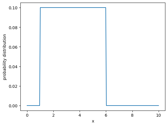
# Let's plot a uniform distribution with a = 1 and b = 6

a = 0 # left endpoint
b = 10 # right endpoint
n = 200 # number fo points

x = np.linspace(a,b,n) #input

uniform = np.piecewise(x, [x < 1, x >= 1,x>6], [0, lambda x: 1/(b-a), 0])

plt.plot(x,uniform)
plt.xlabel('x')
plt.ylabel('probability distribution')
plt.show()
# Let's pull some numbers from a uniform distribution and plot them

# Let's generate 1000 numbers in the range of 1 to 4 from a uniform distribution
numbers = np.random.uniform(1, 4, 1000)

plt.plot(numbers)
plt.xlabel('number')
plt.ylabel('value')
plt.show()
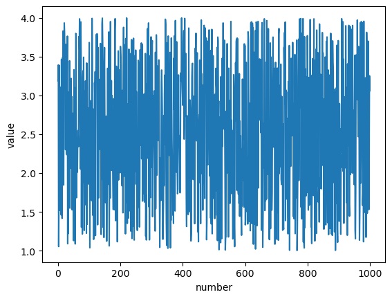
So, why does this not look like the distribution function in the previous plot?
Well, we are not plotting the same thing. In this plot, we are visualizing the 1000 selected numbers in the interval \([1,4]\). To see the distribution, we need count the number of values that have the same output in \([1,4]\) — we need a histogram!
# we will use the histogram plot in matplotlib
buckets = 20 #make 25 bins between 1 and 4.

plt.hist(numbers, buckets, density = True)
plt.ylabel('Probability Distribution')
plt.xlabel('Values')
plt.show()
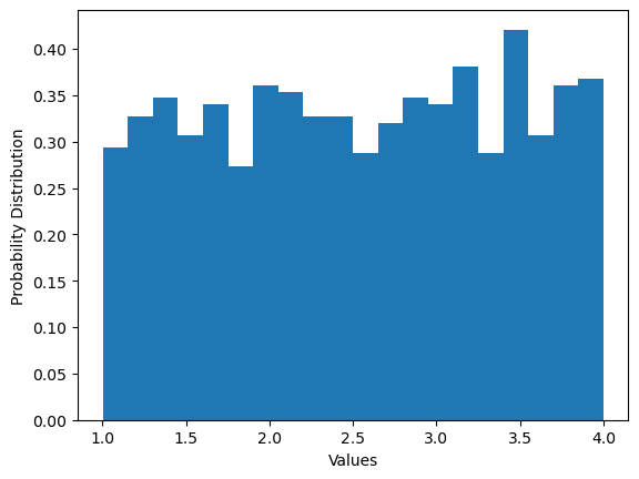
Now, we have a distribution!
Q: How would you change the code blocks above to make it look closer to the definition function?
Normal Distribution#
Plot a normal distribution with \(\mu = 0\) and \(\sigma = 1\).
Use
np.random.normal(mean,variance,n)to randomly sample \(n\) points from a normal distribtion with zero mean, variance of one, and \(n=1000\). Plot the results. Is it a probability distribution? Why or why not? If it is not, what would you need to do to turn it in to a probability distribution?
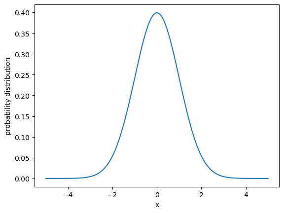
# Let's plot a normal distribution with mean of 0 and standard deviation of 1

mu = 0
sigma = 1

x = np.linspace(-5,5,1000)

normal_dist = 1 / (sigma*np.sqrt(2*np.pi)) * np.exp(-0.5* ((x-mu)/sigma)**2)

plt.plot(x,normal_dist)
plt.xlabel('x')
plt.ylabel('probability distribution')
plt.show()
# We can also generate a normal distribution using the scipy package
from scipy.stats import norm
normal_dist = norm.pdf(x,mu,sigma**2)
# here the input into the norm.pdf function requires variance, not standard deviation, so
# we need to square the sigma value

plt.plot(x,normal_dist)
plt.xlabel('x')
plt.ylabel('probability distribution')
plt.show()
# Now, lets's pull some numbers from a normal distribution and plot them
# Let's generate 1000 numbers with a mean of 0 and variance of 1 from a normal distribution
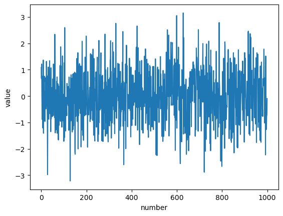
numbers = np.random.normal(0, 1, 1000)
plt.plot(numbers)
plt.xlabel('number')
plt.ylabel('value')
plt.show()
# Like before, we will also create a histogram
buckets = 20 #make 20
plt.hist(numbers, buckets, density = True)
plt.ylabel('Probability Distribution')
plt.xlabel('Values')
plt.show()
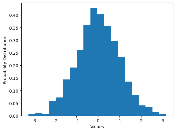
Compare this probability distribution to the function definition. What do you notice? How can you get the shape to be more similar?
Cumulative Distribution#
Using the sample from the normal distirbution above, calculate the cumulative distribution function and plot the curve. Then calculate the probability of \(-1.5 \leq x \leq 2\).
# Let's plot the cumulative distribution for the random numbers we pulled out of the normal distribution
# in the previous code block.

counts, bins = np.histogram(numbers, buckets)
probability = counts/sum(counts)  # this calculates the probability in each bucket
cumulative = np.cumsum(probability) # this sums the probabilities in a cumulative sum

plt.plot(bins[1:],cumulative)
plt.ylabel('Probability Distribution')
plt.xlabel('Values')
plt.show()
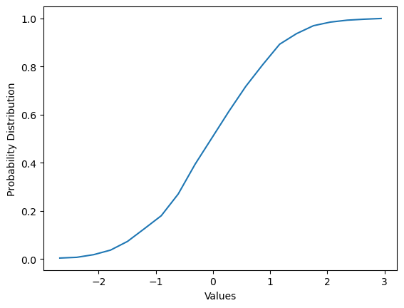
# Here we want P(-1.5 <= x <= 2) = P(x=2) - P(x=-1.5)
# Why P(x=2)-P(x=1.5)? Well, we want the area between -1.5 and 2.  For the cumulative sum
# we calculate from -infinity to the value we are interested in (i.e., the area to the left of the x value).
# So P(x=2) will be -infinity to 2, and then we want to subtract off the area from -infinity to -1.5, or P(x=-1.5)

from scipy.integrate import quad
def normal_pdf(x):
    return (1 / (1*np.sqrt(2*np.pi)) ) * np.exp(-0.5* ((x-0)/1)**2)


Prob_1,error = quad(normal_pdf,-np.inf,-1.5)
Prob_2,error1 = quad(normal_pdf,-np.inf,2)


Total_prob = Prob_2-Prob_1

print(Total_prob)

# alternatively, we could integrate from -1.5 to 2!

Prob_3,error2 = quad(normal_pdf,-1.5,2)
print(Prob_3)
0.9104426667829628
0.9104426667829628
Exponential Distribution#
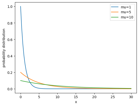
Plot an exponential distribution with means of 1, 5, and 10.
Use
np.random.exponential(scale=mean,size=n)to randomly sample \(n=1000\) points from an exponential distribtion with mean of \(0.5\). Plot the results. Is it a probability distribution? Why or why not? If it is not, what would you need to do to turn it in to a probability distribution?
# Let's plot the exponential distribution with means of 1,5,10.

x = np.linspace(0,30,100)

def exp_dist(x,mu):
    return (1/mu)*np.exp(-(1/mu)*x)

plt.plot(x,exp_dist(x,1),label='mu=1')
plt.plot(x,exp_dist(x,5),label='mu=5')
plt.plot(x,exp_dist(x,10),label='mu=10')
plt.xlabel('x')
plt.ylabel('probability distribution')
plt.legend()
plt.show()
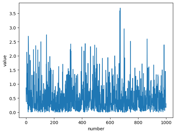
# Now, lets's pull some numbers from an exponential distribution and plot them
# Let's generate 1000 numbers with a mean of 0.5 from an exponential distribution
numbers = np.random.exponential(scale=0.5,size=1000)
plt.plot(numbers)
plt.xlabel('number')
plt.ylabel('value')
plt.show()
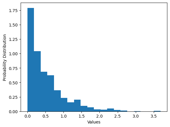
# Like before, we will also create a histogram
buckets = 20 #make 20
plt.hist(numbers, buckets, density = True)
plt.ylabel('Probability Distribution')
plt.xlabel('Values')
plt.show()
In class activity 3#
In your groups, reconfigure your data into a probability density function, and then plot the probability density function.
Calculate the mean and standard deviation of your data using np.mean() and np.std(). Use these values to create a normal distribution of your data set. How does the normal curve match with the “actual” probability density funciton? What do you think would happen if you had more data points?
Some other guiding questions:
How can you check if your probability density function satisfies the definition?
Did you need to normalize your data? Why or why not?
How would you turn your probability density function into a cumulative distribution?
What predictions would you make from your probability density and/or cumulative distribution?