Fast Fourier Transform

The fast Fourier transform (FFT) is an algorithm for efficiently computing the DFT.

Sound signals are commonly sampled at 44.1 kHz (see Wikipedia:Audio sampling). Therefore computing the DFT for a one second sound signal requires the Fourier matrix \(F_N\) for \(N=44100\) which has \(44100^2\) entries (that’s approximately 2 billion). Yikes! We need an efficient algorithm to compute the DFT in practice.

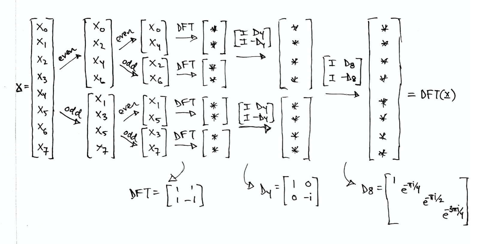
Let \(\boldsymbol{x} \in \mathbb{C}^N\) be a signal of length \(N\) (and assume \(N\) is even). Then

\[\begin{split} \mathrm{DFT}(\boldsymbol{x}) = \renewcommand{\arraystretch}{1.25} \left[ \begin{array}{c} \mathrm{DFT}(\boldsymbol{x}_{\text{even}}) + D_N \mathrm{DFT}(\boldsymbol{x}_{\text{odd}}) \\ \mathrm{DFT}(\boldsymbol{x}_{\text{even}}) - D_N \mathrm{DFT}(\boldsymbol{x}_{\text{odd}}) \end{array} \right] = \left[ \begin{array}{rr} I & D_N \\ I & - D_N \end{array} \right] \left[ \begin{array}{l} \mathrm{DFT}(\boldsymbol{x}_{\text{even}}) \\ \mathrm{DFT}(\boldsymbol{x}_{\text{odd}}) \end{array} \right] \renewcommand{\arraystretch}{1} \end{split}\]

where \(\boldsymbol{x}_{\text{even}}\) and \(\boldsymbol{x}_{\text{odd}}\) are vectors of length \(N/2\) consisting of the even and odd indices respectively

\[\begin{split} \boldsymbol{x}_{\text{even}} = \begin{bmatrix} x_0 \\ x_2 \\ \vdots \\ x_{N-2} \end{bmatrix} \hspace{10mm} \boldsymbol{x}_{\text{odd}} = \begin{bmatrix} x_1 \\ x_3 \\ \vdots \\ x_{N-1} \end{bmatrix} \end{split}\]

and

\[\begin{split} D_N = \begin{bmatrix} 1 & & & \\ & \omega_N^{-1} & & \\ & & \ddots & \\ & & & \omega_N^{-(N/2-1)} \end{bmatrix} \end{split}\]

---

Proof. Let \(\boldsymbol{y} = \mathrm{DFT}(\boldsymbol{x})\), look at the \(k\)th entry of \(\boldsymbol{y}\) and split the sum into the even and odd terms

\[\begin{split} \begin{align*} \boldsymbol{y}[k] &= \langle \boldsymbol{x} , \boldsymbol{f}_k \rangle = \sum_{n=0}^{N-1} x_n \omega_N^{-nk} \\ &= \sum_{m=0}^{N/2-1} x_{2m} \omega_N^{-2mk} + \sum_{m=0}^{N/2-1} x_{2m + 1} \omega_N^{-(2m + 1)k} \end{align*} \end{split}\]

See that \(\omega_N^2 = e^{(2 \pi i / N)2} = e^{2 \pi i / (N/2)} = \omega_{N/2}\) and write

\[ \boldsymbol{y}[k]= \sum_{m=0}^{N/2-1} x_{2m} \omega_{N/2}^{-mk} + \omega_N^{-k} \sum_{m=0}^{N/2-1} x_{2m + 1} \omega_{N/2}^{-mk} \]

For \(0 \leq k < N/2\), these are the formulas for DFT of vectors of length \(N/2\) consisting of the even and odd indices respectively

\[\begin{split} \boldsymbol{x}_{\text{even}} = \begin{bmatrix} x_0 \\ x_2 \\ \vdots \\ x_{N-2} \end{bmatrix} \hspace{10mm} \boldsymbol{x}_{\text{odd}} = \begin{bmatrix} x_1 \\ x_3 \\ \vdots \\ x_{N-1} \end{bmatrix} \end{split}\]

Note that

\[\begin{split} \begin{align*} \boldsymbol{y}[k + N/2] &= \sum_{m=0}^{N/2-1} x_{2m} \omega_{N/2}^{-m(k + N/2)} + \omega_N^{-(k+N/2)} \sum_{m=0}^{N/2-1} x_{2m + 1} \omega_{N/2}^{-m(k + N/2)} \\ &= \sum_{m=0}^{N/2-1} x_{2m} \omega_{N/2}^{-mk} \underbrace{\omega_{N/2}^{-mN/2}}_{1} + \omega_N^{-k} \underbrace{\omega_N^{-N/2}}_{-1} \sum_{m=0}^{N/2-1} x_{2m + 1} \omega_{N/2}^{-mk} \underbrace{\omega_{N/2}^{-mN/2}}_{1} \\ &= \sum_{m=0}^{N/2-1} x_{2m} \omega_{N/2}^{-mk} - \omega_N^{-k} \sum_{m=0}^{N/2-1} x_{2m + 1} \omega_{N/2}^{-mk} \end{align*} \end{split}\]

which again are the DFTs of the even and odd parts of \(\boldsymbol{x}\). Put these formulas for \(\boldsymbol{y}\) together to get

\[\begin{split} \boldsymbol{y} = \mathrm{DFT}(\boldsymbol{x}) = \renewcommand{\arraystretch}{1.25} \left[ \begin{array}{c} \mathrm{DFT}(\boldsymbol{x}_{\text{even}}) + D_N \mathrm{DFT}(\boldsymbol{x}_{\text{odd}}) \\ \mathrm{DFT}(\boldsymbol{x}_{\text{even}}) - D_N \mathrm{DFT}(\boldsymbol{x}_{\text{odd}}) \end{array} \right] \renewcommand{\arraystretch}{1} \end{split}\]

where

\[\begin{split} D_N = \begin{bmatrix} 1 & & & \\ & \omega_N^{-1} & & \\ & & \ddots & \\ & & & \omega_N^{-(N/2-1)} \end{bmatrix} \end{split}\]

This form of the fast Fourier transform is called the Cooley-Tukey algorithm. The point is that the DFT computation for a vector of length \(N\) can be compute by the DFT of two smaller vectors of length \(N/2\) which is faster! And we can keep applying the formulas for smaller and smaller vectors until we are computing the DFT for vectors of size 2 only (if \(N\) is a power of 2). For example, to compute \(\mathrm{DFT}(\boldsymbol{x})\) for \(\boldsymbol{x} \in \mathbb{C}^8\) we visualize the procedure

Use the FFT to compute the DFT of the signal

\[\begin{split} \boldsymbol{x} = \left[ \begin{array}{r} 1 \\ 1 \\ 1 \\ 1 \\ -1 \\ -1 \\ -1 \\ -1 \end{array} \right] \end{split}\]

The symmetry in the signal reduces the number of computations even further

\[\begin{split} \begin{array}{cc} \begin{array}{c} \begin{bmatrix} x_0 \\ x_4 \end{bmatrix} = \left[ \begin{array}{r} 1 \\ -1 \end{array} \right] \stackrel{\mathrm{DFT}}{\longrightarrow} \left[ \begin{array}{r} 0 \\ 2 \end{array} \right] \\ \begin{bmatrix} x_2 \\ x_6 \end{bmatrix} = \left[ \begin{array}{r} 1 \\ -1 \end{array} \right] \stackrel{\mathrm{DFT}}{\longrightarrow} \left[ \begin{array}{r} 0 \\ 2 \end{array} \right] \end{array} & \longrightarrow \left[ \begin{array}{c} \left[ \begin{array}{r} 0 \\ 2 \end{array} \right] + \left[ \begin{array}{rr} 1 & \\ & -i \end{array} \right] \left[ \begin{array}{r} 0 \\ 2 \end{array} \right] \\ \left[ \begin{array}{r} 0 \\ 2 \end{array} \right] - \left[ \begin{array}{rr} 1 & \\ & -i \end{array} \right] \left[ \begin{array}{r} 0 \\ 2 \end{array} \right] \end{array} \right] = \left[ \begin{array}{c} 0 \\ 2-2i \\ 0 \\ 2+2i \end{array} \right] \\ \begin{array}{c} \begin{bmatrix} x_1 \\ x_5 \end{bmatrix} = \left[ \begin{array}{r} 1 \\ -1 \end{array} \right] \stackrel{\mathrm{DFT}}{\longrightarrow} \left[ \begin{array}{r} 0 \\ 2 \end{array} \right] \\ \begin{bmatrix} x_3 \\ x_7 \end{bmatrix} = \left[ \begin{array}{r} 1 \\ -1 \end{array} \right] \stackrel{\mathrm{DFT}}{\longrightarrow} \left[ \begin{array}{r} 0 \\ 2 \end{array} \right] \end{array} & \longrightarrow \left[ \begin{array}{c} \left[ \begin{array}{r} 0 \\ 2 \end{array} \right] + \left[ \begin{array}{rr} 1 & \\ & -i \end{array} \right] \left[ \begin{array}{r} 0 \\ 2 \end{array} \right] \\ \left[ \begin{array}{r} 0 \\ 2 \end{array} \right] - \left[ \begin{array}{rr} 1 & \\ & -i \end{array} \right] \left[ \begin{array}{r} 0 \\ 2 \end{array} \right] \end{array} \right] = \left[ \begin{array}{c} 0 \\ 2-2i \\ 0 \\ 2+2i \end{array} \right] \end{array} \end{split}\]

We can write the matrix \(D_8\) as

\[\begin{split} D_8 = \left[ \begin{array}{rrrr} 1 & & & \\ & e^{- \pi i /4} & & \\ & & e^{- \pi i /2} & \\ & & & e^{- 3\pi i /4} \end{array} \right] = \left[ \begin{array}{rrrr} 1 & & & \\ & \frac{1-i}{\sqrt{2}} & & \\ & & -i & \\ & & & \frac{-1-i}{\sqrt{2}} \end{array} \right] \end{split}\]

and then compute

\[\begin{split} \mathrm{DFT}(\boldsymbol{x}) = \left[ \begin{array}{c} \left[ \begin{array}{c} 0 \\ 2-2i \\ 0 \\ 2+2i \end{array} \right] + \left[ \begin{array}{rrrr} 1 & & & \\ & \frac{1-i}{\sqrt{2}} & & \\ & & -i & \\ & & & \frac{-1-i}{\sqrt{2}} \end{array} \right] \left[ \begin{array}{c} 0 \\ 2-2i \\ 0 \\ 2+2i \end{array} \right] \\ \left[ \begin{array}{c} 0 \\ 2-2i \\ 0 \\ 2+2i \end{array} \right] - \left[ \begin{array}{rrrr} 1 & & & \\ & \frac{1-i}{\sqrt{2}} & & \\ & & -i & \\ & & & \frac{-1-i}{\sqrt{2}} \end{array} \right] \left[ \begin{array}{c} 0 \\ 2-2i \\ 0 \\ 2+2i \end{array} \right] \end{array} \right] = \left[ \begin{array}{c} 0 \\ 2 - 2 \left( \sqrt{2} + 1 \right) i \\ 0 \\ 2 - 2 \left( \sqrt{2} - 1 \right) i \\ 0 \\ 2 + 2 \left( \sqrt{2} - 1 \right) i \\ 0 \\ 2 + 2 \left( \sqrt{2} + 1 \right) i \end{array} \right] \end{split}\]

Exercises

Exercise 1. Let \(\boldsymbol{x} = \begin{bmatrix} 1 & -1 & 2 & 1 \end{bmatrix}^T\). Compute \(\mathrm{DFT}(\boldsymbol{x})\) using the fast Fourier transform. Compute \(\mathrm{DFT}(\boldsymbol{x})\) also by \(F_4\) and verify it is the same result.

Exercise 2. Let \(\boldsymbol{x} = \begin{bmatrix} 1 & 1 & 0 & 2 & 1 & 2 & 0 & -1 \end{bmatrix}^T\). Compute \(\mathrm{DFT}(\boldsymbol{x})\) using the fast Fourier transform.