LU Decomposition#
import numpy as np
import scipy.linalg as la
import matplotlib.pyplot as plt
Implementation#
The function scipy.linalg.lu computes the LU decomposition with partial pivoting which is different than the LU decomposition we consider. So let’s write our own Python function called lu to compute the LU decomposition. The function lu returns \(L=I\) and \(U=A\) with a warning message if the LU decomposition of \(A\) does not exist.
def lu(A):
    "Compute LU decomposition of matrix A."
    m,n = A.shape
    L = np.eye(m)
    U = A.copy()
    # Keep track of the row index of the pivot entry
    pivot = 0
    for j in range(0,n):
        # Check if the pivot entry is 0
        if U[pivot,j] == 0:
            if np.any(U[pivot+1:,j]):
                # LU decomposition does not exist if entries below 0 pivot are nonzero
                print("LU decomposition for A does not exist.")
                return np.eye(m),A
            else:
                # All entries below 0 pivot are 0 therefore continue to next column
                # Row index of pivot remains the same
                continue
        # Use nonzero pivot entry to create 0 in each entry below
        for i in range(pivot+1,m):
            c = -U[i,j]/U[pivot,j]
            U[i,:] = c*U[pivot,:] + U[i,:]
            L[i,pivot] = -c
        # Move pivot to the next row
        pivot += 1
    return L,U
Let’s verify our function works:
A = np.array([[2.,1.,1.],[2.,0.,2.],[4.,3.,4.]])
A
array([[2., 1., 1.],
       [2., 0., 2.],
       [4., 3., 4.]])
L,U = lu(A)
L
array([[ 1.,  0.,  0.],
       [ 1.,  1.,  0.],
       [ 2., -1.,  1.]])
U
array([[ 2.,  1.,  1.],
       [ 0., -1.,  1.],
       [ 0.,  0.,  3.]])
L@U
array([[2., 1., 1.],
       [2., 0., 2.],
       [4., 3., 4.]])
Success! Let’s try an example where we know the LU decomposition does not exist:
A = np.array([[0.,1.],[1.,0.]])
L,U = lu(A)
LU decomposition for A does not exist.
L
array([[1., 0.],
       [0., 1.]])
U
array([[0., 1.],
       [1., 0.]])
Now let’s try an example with some zeros along the diagonal of the \(U\):
A = np.array([[2,2,-2,4,2],[1,-1,0,2,1],[3,1,-2,6,3],[1,3,-2,2,1]])
A
array([[ 2,  2, -2,  4,  2],
       [ 1, -1,  0,  2,  1],
       [ 3,  1, -2,  6,  3],
       [ 1,  3, -2,  2,  1]])
L,U = lu(A)
L
array([[ 1. ,  0. ,  0. ,  0. ],
       [ 0.5,  1. ,  0. ,  0. ],
       [ 1.5,  1. ,  1. ,  0. ],
       [ 0.5, -1. ,  0. ,  1. ]])
U
array([[ 2,  2, -2,  4,  2],
       [ 0, -2,  1,  0,  0],
       [ 0,  0,  0,  0,  0],
       [ 0,  0,  0,  0,  0]])
L@U
array([[ 2.,  2., -2.,  4.,  2.],
       [ 1., -1.,  0.,  2.,  1.],
       [ 3.,  1., -2.,  6.,  3.],
       [ 1.,  3., -2.,  2.,  1.]])
Success! Let’s do onemore example:
A = np.array([[1,1,-1,2,1,3],[2,5,-5,5,2,10],[-1,2,-2,-1,4,2],[3,3,-3,6,-7,5],[-4,20,-20,0,1,15]])
A
array([[  1,   1,  -1,   2,   1,   3],
       [  2,   5,  -5,   5,   2,  10],
       [ -1,   2,  -2,  -1,   4,   2],
       [  3,   3,  -3,   6,  -7,   5],
       [ -4,  20, -20,   0,   1,  15]])
L,U = lu(A)
L
array([[ 1.,  0.,  0.,  0.,  0.],
       [ 2.,  1.,  0.,  0.,  0.],
       [-1.,  1.,  1.,  0.,  0.],
       [ 3., -0., -2.,  1.,  0.],
       [-4.,  8.,  1.,  3.,  1.]])
U
array([[ 1,  1, -1,  2,  1,  3],
       [ 0,  3, -3,  1,  0,  4],
       [ 0,  0,  0,  0,  5,  1],
       [ 0,  0,  0,  0,  0, -2],
       [ 0,  0,  0,  0,  0,  0]])
L@U
array([[  1.,   1.,  -1.,   2.,   1.,   3.],
       [  2.,   5.,  -5.,   5.,   2.,  10.],
       [ -1.,   2.,  -2.,  -1.,   4.,   2.],
       [  3.,   3.,  -3.,   6.,  -7.,   5.],
       [ -4.,  20., -20.,   0.,   1.,  15.]])
Example#
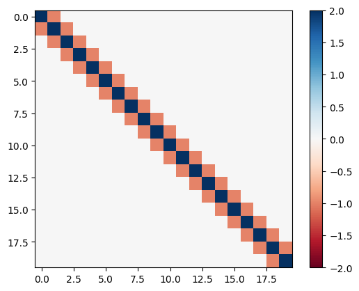
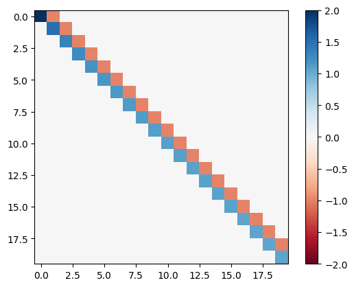
Consider the \(N\) by \(N\) matrix
Compute the solution of the system \(A \mathbf{x} = \mathbf{b}\) for
by computing the LU decomposition and using the function scipy.linalg.solve_triangular.
N = 20
A1 = 2*np.eye(N)
A2 = np.diag(-np.ones(N-1),1)
A = A1 + A2 + A2.T
plt.imshow(A,cmap='RdBu'), plt.clim([-2,2])
plt.colorbar()
plt.show()
Compute the LU decomposition \(A=LU\) and visualize the matrices \(L\) and \(U\):
L,U = lu(A)
plt.imshow(L,cmap='RdBu'), plt.clim([-2,2]), plt.colorbar()
plt.show()
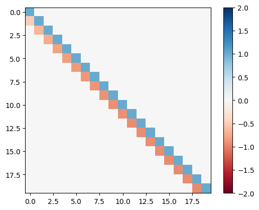
plt.imshow(U,cmap='RdBu'), plt.clim([-2,2]), plt.colorbar()
plt.show()
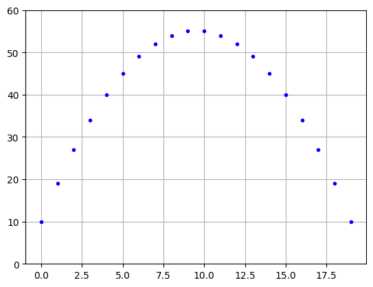
Solve the systems \(L \boldsymbol{y} = \boldsymbol{b}\) and \(U \boldsymbol{x} = \boldsymbol{y}\), then plot the solution \(\boldsymbol{x}\):
b = np.ones([N,1])
y = la.solve_triangular(L,b,lower=True)
x = la.solve_triangular(U,y,lower=False)
plt.plot(x,'b.'), plt.grid(True), plt.ylim([0,60])
plt.show()