Singular Value Decomposition

If \(A\) is any \(m \times n\) matrix, then \(AA^T\) and \(A^TA\) are symmetric matrices therefore both are orthogonally diagonalizable, \(AA^T = PD_1P^T\) and \(A^TA = QD_2Q^T\), and these decompositions lead to the singular value decomposition \(A = P \Sigma Q^T\) where \(\Sigma\) is a diagonal \(m \times n\) matrix containing the singular values (the square roots of the eigenvalues in \(D_1\) and \(D_2\)).

SVD Construction

Throughout this section \(A\) is a real \(m \times n\) matrix.

All eigenvalues of \(AA^T\) and \(A^TA\) are non-negative (that is, \(\lambda \geq 0\)).

Proof

Let \(\lambda\) be an eigenvalue of \(AA^T\) with eigenvector \(\boldsymbol{p}\). Compute

\[ \| A^T \boldsymbol{p} \|^2 = \langle A^T \boldsymbol{p} , A^T \boldsymbol{p} \rangle = \langle \boldsymbol{p}, AA^T \boldsymbol{p} \rangle = \lambda \langle \boldsymbol{p} , \boldsymbol{p} \rangle = \lambda \| \boldsymbol{p} \|^2 \]

Since \(\boldsymbol{p}\) is a nonzero vector, we can write

\[ \lambda = \frac{\| A^T \boldsymbol{p} \|^2}{\| \boldsymbol{p} \|^2} \]

therefore \(\lambda\) is a real number squared and must be non-negative. The same calculation works for \(A^TA\).

Let \(\lambda\) be a positive eigenvalue of \(AA^T\) with unit eigenvector \(\boldsymbol{p}\). Then \(\lambda\) is an eigenvalue of \(A^TA\) with unit eigenvector

\[ \boldsymbol{q} = \frac{1}{\sigma} A^T \boldsymbol{p} \ , \ \ \sigma = \sqrt{\lambda} \]

Conversely, let \(\lambda\) be a positive eigenvalue of \(A^TA\) with (unit) eigenvector \(\boldsymbol{q}\). Then \(\lambda\) is an eigenvalue of \(AA^T\) with eigenvector

\[ \boldsymbol{p} = \frac{1}{\sigma} A \boldsymbol{q} \ , \ \ \sigma = \sqrt{\lambda} \]

Proof

Compute

\[ A^TA \boldsymbol{q} = \frac{1}{\sqrt{\lambda}} A^T A A^T \boldsymbol{p} = \frac{1}{\sqrt{\lambda}} A^T A A^T \boldsymbol{p} = \sqrt{\lambda} A^T \boldsymbol{p} = \lambda \boldsymbol{q} \]

Therefore \(\boldsymbol{q}\) is an eigenvector for \(A^TA\) with eigenvalue \(\lambda\). Now let’s verify it is a unit vector. Compute

\[ \| \boldsymbol{q} \|^2 = \langle \boldsymbol{q} , \boldsymbol{q} \rangle = \frac{1}{\sigma^2} \langle A^T \boldsymbol{p} , A^T \boldsymbol{p} \rangle = \frac{1}{\lambda} \langle \boldsymbol{p} , AA^T \boldsymbol{p} \rangle = \langle \boldsymbol{p} , \boldsymbol{p} \rangle = 1 \]

Similar computations prove the second statement regarding \(\boldsymbol{p} = \displaystyle \frac{1}{\sigma} A \boldsymbol{q}\).

The formulas relating \(\boldsymbol{p}\) and \(\boldsymbol{q}\) above for \(\lambda > 0\) imply that the multiplicity of the eigenvalue \(\lambda\) for \(AA^T\) is equal to the multiplicity of the eigenvalue \(\lambda\) for \(A^TA\).

The matrices \(AA^T\) and \(A^TA\) have the same set of positive eigenvalues. Label the eigenvalues in decreasing order \(\lambda_1 \geq \lambda_2 \geq \cdots \geq \lambda_r > 0\). The singular values of \(A\) are

\[ \sigma_i = \sqrt{\lambda_i} \ \ , \ \ i=1,\dots,r \]

\(N(AA^T) = N(A^T)\) and \(N(A^TA) = N(A)\).

Proof

If \(\boldsymbol{v} \in N(A^T)\) then \(AA^T \boldsymbol{v} = 0\) and so \(\boldsymbol{v} \in N(AA^T)\) and so \(N(A^T) \subset N(AA^T)\).

Now let \(\boldsymbol{v} \in N(AA^T)\). Compute

\[ \| A^T \boldsymbol{v} \|^2 = \langle A^T \boldsymbol{v} , A^T \boldsymbol{v} \rangle = \langle \boldsymbol{v} , AA^T \boldsymbol{v} \rangle = 0 \]

Therefore \(A^T \boldsymbol{v} = 0\) and \(\boldsymbol{v} \in N(A^T)\) and so \(N(AA^T) \subset N(A^T)\). Finally, we conclude \(N(AA^T) = N(A^T)\).

Similar computations prove the statement \(N(A^TA) = N(A)\).

Let \(A\) be an \(m \times n\) matrix and let \(\sigma_1 \geq \sigma_2 \geq \cdots \geq \sigma_r > 0\) be the singular values of \(A\). There exist orthogonal matrices \(P\) and \(Q\) such that

\[\begin{split} A = P \Sigma Q^T \hspace{5mm} \text{where} \hspace{5mm} \Sigma = \left[ \begin{array}{ccc|c} \sigma_1 & & & \\ & \ddots & & \boldsymbol{0} \\ & & \sigma_r & \\ \hline & \boldsymbol{0} & & \boldsymbol{0} \end{array} \right]_{m \times n} \end{split}\]

Proof

The matrix \(A^TA\) is a \(n \times n\) symmetric matrix and is therefore orthogonally diagonalizable. Let \(\boldsymbol{q}_1,\dots,\boldsymbol{q}_n\) be orthonormal eigenvectors of \(A^TA\) chosen in order such that

\[ A^TA \boldsymbol{q}_i = \sigma_i^2 \boldsymbol{q}_i \ \ , \ \ i =1,\dots,r \hspace{15mm} A^TA \boldsymbol{q}_i = \boldsymbol{0} \ \ , \ \ i =r+1,\dots,n \]

Note that \(\boldsymbol{q}_{r+1},\dots,\boldsymbol{q}_r \in N(A)\). Let \(Q\) be the orthogonal matrix

\[\begin{split} Q = \begin{bmatrix} & & \\ \boldsymbol{q}_1 & \cdots & \boldsymbol{q}_n \\ & & \end{bmatrix} \end{split}\]

The matrix \(AA^T\) is a \(m \times m\) symmetric matrix and is therefore orthogonally diagonalizable. Let

\[ \boldsymbol{p}_i = \frac{1}{\sigma_i} A \boldsymbol{q}_i \ \ , \ \ i = 1,\dots,r \]

Each \(\boldsymbol{p}_1,\dots,\boldsymbol{p}_r\) is a unit eigenvector for \(AA^T\) with eigenvalue \(\lambda_i\). Find an orthonormal basis \(\boldsymbol{p}_{r+1},\dots,\boldsymbol{p}_m\) of the nullspace \(N(A^T)\). Then \(\boldsymbol{p}_1,\dots,\boldsymbol{p}_m\) are orthonormal eigenvectors for \(AA^T\). Define the orthogonal matrix

\[\begin{split} P = \begin{bmatrix} & & \\ \boldsymbol{p}_1 & \cdots & \boldsymbol{p}_m \\ & & \end{bmatrix} \end{split}\]

Compute

\[\begin{split} \begin{align*} AQ &= \begin{bmatrix} & & & & & \\ A \boldsymbol{q}_1 & \cdots & A\boldsymbol{q}_r & A\boldsymbol{q}_{r+1} & \cdots & A\boldsymbol{q}_n \\ & & & & & \end{bmatrix} \\ &= \begin{bmatrix} & & & & & \\ \sigma_1 \boldsymbol{p}_1 & \cdots & \sigma_r \boldsymbol{p}_r & \boldsymbol{0} & \cdots & \boldsymbol{0} \\ & & & & & \end{bmatrix} \end{align*} \end{split}\]

Finally, compute

\[\begin{split} \begin{align*} P \Sigma &= \begin{bmatrix} & & & & & \\ \boldsymbol{p}_1 & \cdots & \boldsymbol{p}_r & \boldsymbol{p}_{r+1} & \cdots & \boldsymbol{p}_n \\ & & & & & \end{bmatrix} \left[ \begin{array}{ccc|c} \sigma_1 & & & \\ & \ddots & & \boldsymbol{0} \\ & & \sigma_r & \\ \hline & \boldsymbol{0} & & \boldsymbol{0} \end{array} \right] \\ &= \begin{bmatrix} & & & & & \\ \sigma_1 \boldsymbol{p}_1 & \cdots & \sigma_r \boldsymbol{p}_r & \boldsymbol{0} & \cdots & \boldsymbol{0} \\ & & & & & \end{bmatrix} \end{align*} \end{split}\]

Therefore \(AQ = P \Sigma\) and so \(A = P \Sigma Q^T\).

The equation \(A = P \Sigma Q^T\) is called the singular value decomposition of \(A\), the diagonal entries of \(\Sigma\) are the singular values, the columns of \(P\) are called the left singular vectors and the columns of \(Q\) are called the right singular vectors.

In the construction of the SVD, we may chose to first construct either \(P\) or \(Q\). The connection between the columns for \(i = 1,\dots,r\) are given by the equations:

\[\begin{split} \begin{align*} \boldsymbol{q}_i &= \frac{1}{\sigma_i} A^T \boldsymbol{p}_i & A^TA \boldsymbol{q}_i &= \sigma_i^2 \boldsymbol{q}_i & \| \boldsymbol{q}_i \| &= 1 \\ \boldsymbol{p}_i &= \frac{1}{\sigma_i} A \boldsymbol{q}_i & AA^T \boldsymbol{p}_i &= \sigma_i^2 \boldsymbol{p}_i & \| \boldsymbol{p}_i \| &= 1 \end{align*} \end{split}\]

Construct the SVD for

\[\begin{split} A = \left[ \begin{array}{rr} 1 & 1 \\ 1 & -1 \\ 0 & 1 \end{array} \right] \end{split}\]

Since \(A^TA\) is a smaller matrix, let us first construct \(Q\). Compute

\[\begin{split} A^TA = \begin{bmatrix} 2 & 0 \\ 0 & 3 \end{bmatrix} \end{split}\]

Therefore \(\sigma_1 = \sqrt{3}\) and \(\sigma_2 = \sqrt{2}\). By inspection, we find

\[\begin{split} \boldsymbol{q}_1 = \begin{bmatrix} 0 \\ 1 \end{bmatrix} \hspace{5mm} \boldsymbol{q}_2 = \begin{bmatrix} 1 \\ 0 \end{bmatrix} \hspace{5mm} \Rightarrow \hspace{5mm} Q = \begin{bmatrix} 0 & 1 \\ 1 & 0 \end{bmatrix} \end{split}\]

Construct the matrix \(P\)

\[\begin{split} \boldsymbol{p}_1 = \frac{1}{\sigma_1} A\boldsymbol{q}_1 = \frac{1}{\sqrt{3}} \left[ \begin{array}{r} 1 \\ -1 \\ 1 \end{array} \right] \hspace{5mm} \boldsymbol{p}_2 = \frac{1}{\sigma_2} A\boldsymbol{q}_2 = \frac{1}{\sqrt{2}} \left[ \begin{array}{r} 1 \\ 1 \\ 0 \end{array} \right] \end{split}\]

Extend to an orthonormal basis of \(\mathbb{R}^3\) by finding \(\boldsymbol{p}_3\) orthogonal to \(\boldsymbol{p}_1\) and \(\boldsymbol{p}_2\). There are different ways of doing this. Setup equations \(\langle \boldsymbol{p}_1 , \boldsymbol{p}_3 \rangle = 0\) and \(\langle \boldsymbol{p}_2 , \boldsymbol{p}_3 \rangle = 0\) in a linear system and solve

\[\begin{split} \left[ \begin{array}{rrr|r} 1 & -1 & \phantom{+}1 & 0 \\ 1 & 1 & 0 & 0 \end{array} \right] \hspace{5mm} \Rightarrow \hspace{5mm} \boldsymbol{p}_3 = \frac{1}{\sqrt{6}} \left[ \begin{array}{r} -1 \\ 1 \\ 2 \end{array} \right] \end{split}\]

Therefore the SVD is given by

\[\begin{split} A = P \Sigma Q^T = \left[ \begin{array}{rcr} 1/\sqrt{3} & 1/\sqrt{2} & -1/\sqrt{6} \\ -1/\sqrt{3} & 1/\sqrt{2} & 1/\sqrt{6} \\ 1/\sqrt{3} & 0 & 2/\sqrt{6} \end{array} \right] \left[ \begin{array}{rr} \sqrt{3} & 0 \\ 0 & \sqrt{2} \\ 0 & 0 \end{array} \right] \begin{bmatrix} 0 & 1 \\ 1 & 0 \end{bmatrix}^T \end{split}\]

Corollaries of SVD

Let \(A = P \Sigma Q^T\).

• \(N(A) = \mathrm{span} \{ \boldsymbol{q}_{r+1},\dots,\boldsymbol{q}_n \}\)

• \(R(A) = \mathrm{span} \{ \boldsymbol{p}_1,\dots,\boldsymbol{p}_r \}\)

• \(N(A^T) = \mathrm{span} \{ \boldsymbol{p}_{r+1},\dots,\boldsymbol{p}_m \}\)

• \(R(A^T) = \mathrm{span} \{ \boldsymbol{q}_1,\dots,\boldsymbol{q}_r \}\)

• \(\mathrm{rank}(A) = r\)

Let \(\sigma_1\) be the largest singular value of \(A\). Then \(\| A \| = \sigma_1\).

Proof

Since \(P\) is an orthogonal matrix \(\| P \Sigma Q^T \boldsymbol{x} \| = \| \Sigma Q^T \boldsymbol{x} \|\) for all \(\boldsymbol{x}\). Compute from the definition

\[ \| A \| = \max_{\boldsymbol{x} \not= 0} \| A \boldsymbol{x} \| = \max_{\boldsymbol{x} \not= 0} \| P \Sigma Q^T \boldsymbol{x} \| = \max_{\boldsymbol{x} \not= 0} \| \Sigma Q^T \boldsymbol{x} \| \]

Let \(\boldsymbol{y} = Q^T \boldsymbol{x}\) and write the equation

\[ \| A \| = \max_{\boldsymbol{y} \not= 0} \| \Sigma \boldsymbol{y} \| = \| \Sigma \| \]

Since \(\Sigma\) is a diagonal matrix we know that \(\| \Sigma \|\) is equal to the absolute value of the maximum of the diagonal entries and so \(\| A \| = \sigma_1\).

Let \(A\) be a \(n \times n\) invertible matrix. Let \(\sigma_1\) be the largest singular value of \(A\) and let \(\sigma_n\) be the smallest. Then \(\| A^{-1} \| = 1/\sigma_n\) and \(\mathrm{cond}(A) = \frac{\sigma_1}{\sigma_n}\).

Proof

Let \(\sigma_1 \geq \cdots \geq \sigma_n\) be the singular values of \(A\). The singular values of \(A^{-1}\) in decreasing order are \(1/\sigma_n \geq \cdots \geq 1/\sigma_1\) therefore \(\| A^{-1} \| = 1/\sigma_n\) and finally

\[ \mathrm{cond}(A) = \| A \| \| A^{-1} \| = \frac{\sigma_1}{\sigma_n} \]

Principal Component Analysis

Let \(\boldsymbol{x}_1 , \dots , \boldsymbol{x}_n \in \mathbb{R}^p\) (viewed as row vectors) and let \(X\) be the \(n \times p\) data matrix where row \(k\) is given by \(\boldsymbol{x}_k\). Assume the data is normalized such that the mean value of each column of \(X\) is 0. The unit vector \(\boldsymbol{w}_1\) which maximizes the sum

\[ \sum_{i=1}^n \langle \boldsymbol{x}_i , \boldsymbol{w}_1 \rangle^2 = \| X \boldsymbol{w}_1 \|^2 \]

is called the first weight vector of \(X\) (see Wikipedia:Principal component analysis). More generally, given weight vectors \(\boldsymbol{w}_1 , \dots, \boldsymbol{w}_{k-1}\), the \(k\)th weight vector of \(X\) is the unit vector \(\boldsymbol{w}_k\) which maximizes

\[ \| X_k \boldsymbol{w}_k \|^2 \]

where \(X_k\) is the projection of the data matrix \(X\) onto \(\mathrm{span} \{ \boldsymbol{w}_1 , \dots, \boldsymbol{w}_{k-1} \}^{\perp}\)

\[ X_k = X - \sum_{j=1}^{k-1} X \boldsymbol{w}_j \boldsymbol{w}_j^T \]

The projection coefficient \(\langle \boldsymbol{x}_i , \boldsymbol{w}_k \rangle\) is called the \(k\)th principal component of a data vector \(\boldsymbol{x}_i\).

Each \(\langle \boldsymbol{x}_k , \boldsymbol{w}_1 \rangle^2\) is the length squared of the orthogonal projection of \(\boldsymbol{x}_k\) onto \(\boldsymbol{w}_1\). Therefore the first weight vector \(\boldsymbol{w}_1\) points in the direction which captures the most information (ie. the maximum variance) of the data, and the second weight vector \(\boldsymbol{w}_2\) is orthogonal to \(\boldsymbol{w}_1\).

The weight vectors \(\boldsymbol{w}_1 , \dots , \boldsymbol{w}_p\) are the right singular vectors of the matrix \(X\). In other words, let \(X = P \Sigma Q^T\) be a singular value decomposition of \(X\) and let \(\boldsymbol{q}_1, \dots, \boldsymbol{q}_p\) be the columns of \(Q\) corresponding to singular values \(\sigma_1 > \cdots > \sigma_p > 0\). Then \(\boldsymbol{w}_1 = \boldsymbol{q}_1 , \dots , \boldsymbol{w}_p = \boldsymbol{q}_p\).

Proof

Let \(X = P \Sigma Q^T\) be a singular value decomposition of \(X\). We know that \(\| X \| = \sigma_1\) where \(\sigma_1\) is the largest singular value of \(X\) and therefore the first weight vector will satisfy \(\| X \boldsymbol{w}_1 \| = \sigma_1\). Note that

\[ \| X \boldsymbol{w} \| = \| P \Sigma Q^T \boldsymbol{w} \| = \| \Sigma Q^T \boldsymbol{w} \| \]

Since \(\Sigma\) is diagonal with diagonal entires \(\sigma_1 \geq \cdots \geq \sigma_p\), the maximum value of \(\| X \boldsymbol{w} \|\) occurs when

\[\begin{split} Q^T \boldsymbol{w} = \begin{bmatrix} 1 \\ 0 \\ \vdots \\ 0 \end{bmatrix} \end{split}\]

therefore \(\boldsymbol{w}_1 = \boldsymbol{q}_1\). For general \(k\), note that the singular value decomposition \(X_k = P_k \Sigma_k Q^T_k\) is obtained from \(X\) by removing the singular values \(\sigma_1,\dots,\sigma_{k-1}\). Therefore the largest singular value of \(X_k\) is \(\sigma_k\) with corresponding right singular vector \(\boldsymbol{q}_k\) and therefore \(\boldsymbol{w}_k = \boldsymbol{q}_k\).

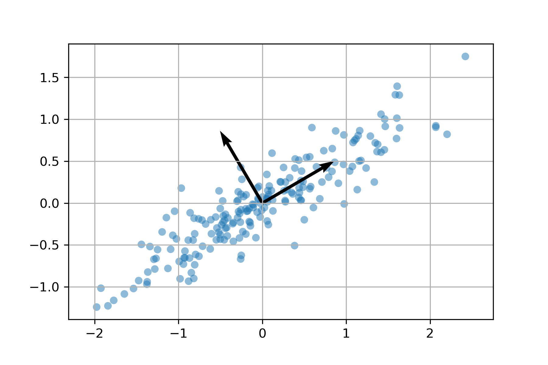
Find the first weight vector for the data given in the image below.

We expect

\[\begin{split} \boldsymbol{w}_1 = \begin{bmatrix} 1/\sqrt{2} \\ 1/\sqrt{2} \end{bmatrix} \end{split}\]

since that direction clearly captures the most information. Form the data matrix

\[\begin{split} X^T = \left[ \begin{array}{rrrrrrr} -2 & -1 & -1 & \phantom{+}0 & 1 & \phantom{+}1 & 2 \\ -2 & -1 & 1 & 0 & -1 & 1 & 2 \end{array} \right] \end{split}\]

We don’t need to compute the full SVD of \(X\) but just the first right singular vector. Compute

\[\begin{split} X^T X = \begin{bmatrix} 12 & 8 \\ 8 & 12 \end{bmatrix} \end{split}\]

The characteristic polynomial of \(X^TX\) is

\[ \det (xI - X^TX) = (x-12)^2 - 8^2 = x^2 - 24x + 80 = (x - 4)(x - 20) \]

The right singular vector \(\boldsymbol{q}_1\) for \(X\) is a unit eigenvector for \(X^TX\) for the eigenvalue \(\lambda_1 = 20\). Compute

\[\begin{split} ( X^T X - 20 I)\boldsymbol{w}_1 = \boldsymbol{0} \ \ \Rightarrow \ \ \left[ \begin{array}{rr|r} -8 & 8 & 0 \\ 8 & -8 & \phantom{+}0 \end{array} \right] \ \ \Rightarrow \ \ \boldsymbol{w}_1 = \frac{1}{\sqrt{2}} \begin{bmatrix} 1 \\ 1 \end{bmatrix} \end{split}\]

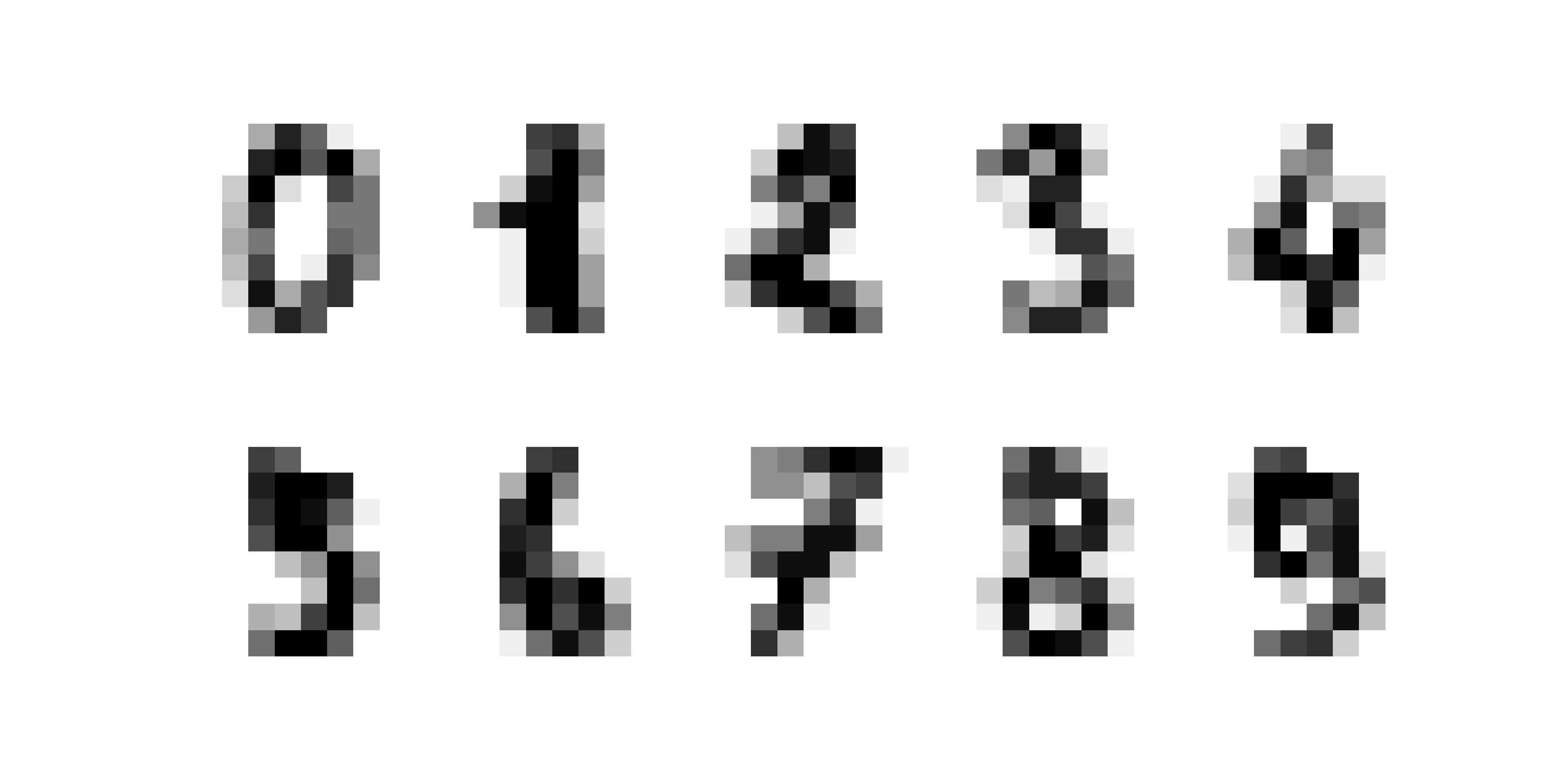
The digits dataset from sklearn is a \(1797 \times 64\) data matrix \(X\) such that each row represents an \(8 \times 8\) pixel image of a handwritten number. The first 10 rows of X (reshaped from vectors of length 64 to \(8 \times 8\) matrices to visualize) are:

Compute the first 2 weight vectors and find (again \(\boldsymbol{w}_1,\boldsymbol{w}_2\) reshaped from vectors of length 64 to \(8 \times 8\) matrices to visualize)

We can see \(\boldsymbol{w}_1\) looks like a 3 and \(\boldsymbol{w}_2\) looks like 0. Project the entire dataset onto these weight vectors and label each data point by a color according to the digit:

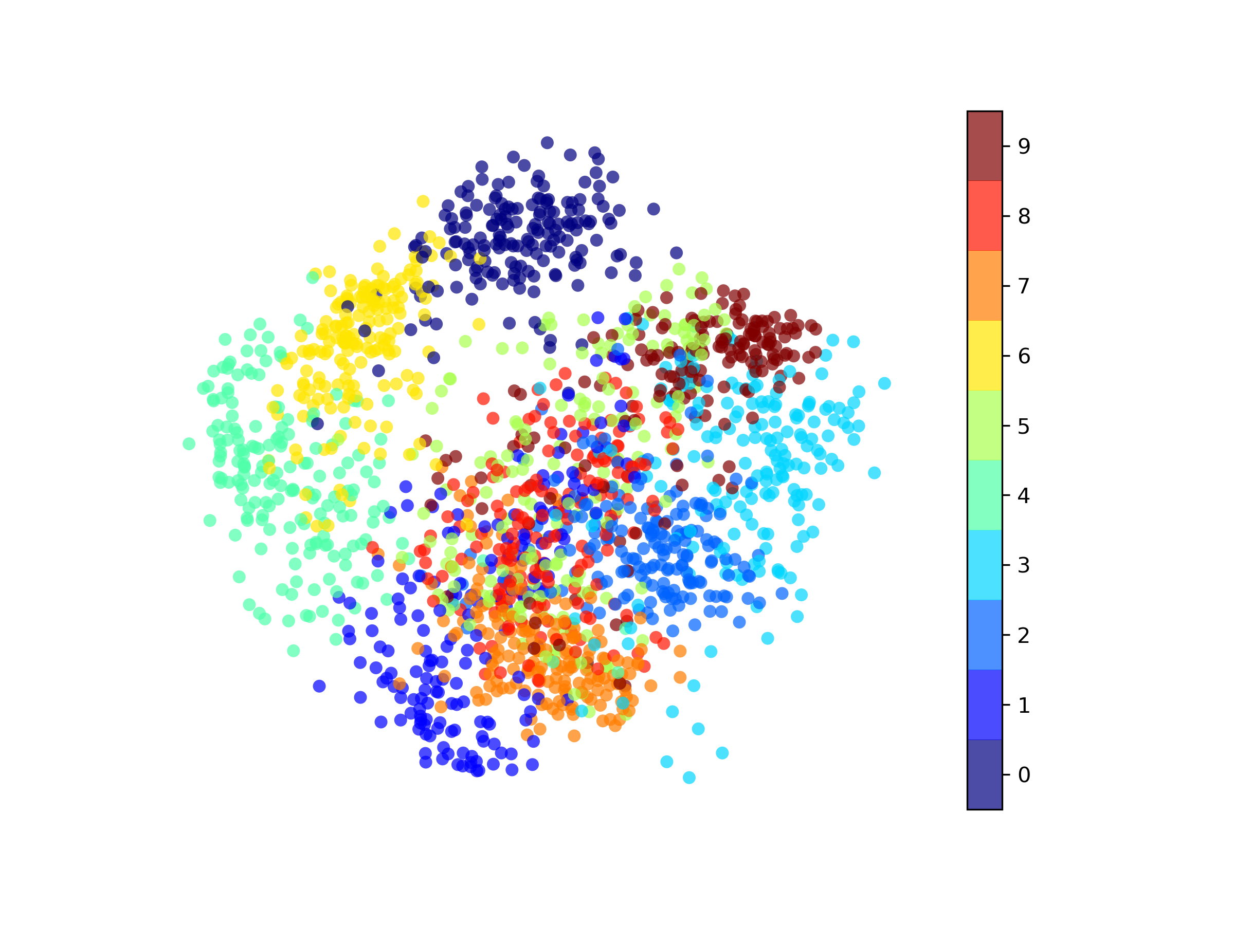
We can see that the 3s are to the right in the horizontal direction since these points most similar to \(\boldsymbol{w}_1\), and the 0s are at the top in the vertical direction since these points most similar to \(\boldsymbol{w}_2\). We can make other interesting observations such as the 4s are opposite to the 3s and orthogonal to 0s, and 7s and 1s are opposite to 0s and orthogonal to 3s.

Pseudoinverse and Least Squares

Let \(A\) be a \(m \times n\) matrix such that \(\mathrm{rank}(A) = r\) and let \(A = P \Sigma Q^T\). The pseudoinverse of \(A\) is \(A^+ = Q \Sigma^+ P^T\) where

\[\begin{split} \Sigma^+ = \left[ \begin{array}{ccc|c} \sigma_1^{-1} & & & \\ & \ddots & & \boldsymbol{0} \\ & & \sigma_r^{-1} & \\ \hline & \boldsymbol{0} & & \boldsymbol{0} \end{array} \right]_{n \times m} \end{split}\]

If \(A\) is invertible, then \(A^+ = A^{-1}\).

Let \(A\) be an \(m \times n\) matrix with \(\mathrm{rank}(A) = n\) and let \(\boldsymbol{b} \in \mathbb{R}^m\). The least squares approximation of the system \(A \boldsymbol{x} \cong \boldsymbol{b}\) is given by \(\boldsymbol{x} = A^+ \boldsymbol{b}\).

Proof

Let \(P^T \boldsymbol{b} = \boldsymbol{c}\) and write

\[\begin{split} \boldsymbol{c} = \begin{bmatrix} c_1 \\ \vdots \\ c_m \end{bmatrix} \in \mathbb{R}^m \end{split}\]

Since \(P\) is an orthogonal matrix we have

\[ \| A \boldsymbol{x} - \boldsymbol{b} \| = \| P (\Sigma Q^T \boldsymbol{x} - P^T \boldsymbol{b} ) \| = \| \Sigma Q^T \boldsymbol{x} - \boldsymbol{c} \| \]

The matrix \(\Sigma\) is of the form

\[\begin{split} \Sigma = \left[ \begin{array}{ccc} \sigma_1 & & \\ & \ddots & \\ & & \sigma_n \\ \hline \boldsymbol{0} & \cdots & \boldsymbol{0} \end{array} \right]_{m \times n} \end{split}\]

and so only the first \(n\) entries of \(\Sigma \boldsymbol{v}\) are nonzero for any vector \(\boldsymbol{v} \in \mathbb{R}^n\). Therefore the minimum value \(\| A \boldsymbol{x} - \boldsymbol{b} \| = \| \Sigma Q^T \boldsymbol{x} - \boldsymbol{c} \|\) occurs when

\[\begin{split} \Sigma Q^T \boldsymbol{x} = \begin{bmatrix} c_1 \\ \vdots \\ c_n \\ \boldsymbol{0} \end{bmatrix} \end{split}\]

and so \(\boldsymbol{x} = Q \Sigma^+ \boldsymbol{c}\). Altogether, we have \(\boldsymbol{x} = Q \Sigma^+ P^T \boldsymbol{b} = A^+ \boldsymbol{b}\).

\(AA^+\) is the projection matrix onto \(R(A)\) and \(A^+A\) is the projection onto \(R(A^T)\).

Proof

Compute \(AA^+ = P \Sigma Q^T Q \Sigma^+ P^T = P \Sigma \Sigma^+ P^T\) and note

\[\begin{split} \Sigma \Sigma^+ = \left[ \begin{array}{c|c} I_r & \boldsymbol{0} \\ \hline \boldsymbol{0} & \boldsymbol{0} \end{array} \right]_{m \times m} \end{split}\]

where \(I_r\) is the identity of matrix of size \(r\). Let

\[\begin{split} P_r = \begin{bmatrix} & & \\ \boldsymbol{p}_1 & \cdots & \boldsymbol{p}_r \\ & & \end{bmatrix} \end{split}\]

where \(\boldsymbol{p}_1,\dots,\boldsymbol{p}_r\) are the first \(r\) columns of \(P\). By definition, the projection matrix onto \(R(A)\) is \(P_r P_r^T\) and we want to show that \(P \Sigma \Sigma^+ P^T = P_r P_r^T\). Equivalently, we can show that \(P \Sigma \Sigma^+ = P_r P_r^T P\). Multiplying everything out shows that

\[\begin{split} P \Sigma \Sigma^+ = \begin{bmatrix} & & & & & \\ \boldsymbol{p}_1 & \cdots & \boldsymbol{p}_r & \boldsymbol{0} & \cdots & \boldsymbol{0} \\ & & & & & \end{bmatrix} \end{split}\]

and also

\[\begin{split} P_r P_r^T P = \begin{bmatrix} & & & & & \\ \boldsymbol{p}_1 & \cdots & \boldsymbol{p}_r & \boldsymbol{0} & \cdots & \boldsymbol{0} \\ & & & & & \end{bmatrix} \end{split}\]

therefore \(AA^+ = P_rP_r^T\) is the projection matrix onto \(R(A)\). Similar computations show that \(A^+A\) is the projection onto \(R(A^T)\).

\(AA^+A = A\) and \(A^+AA^+=A^+\).

Proof

Compute

\[\begin{split} \begin{align*} AA^+A &= P \Sigma Q^T Q \Sigma^+ P^T P \Sigma Q^T \\ &= P \Sigma \Sigma^+ \Sigma Q^T \\ &= P \Sigma \left[ \begin{array}{c|c} I_r & \boldsymbol{0} \\ \hline \boldsymbol{0} & \boldsymbol{0} \end{array} \right] Q^T \\ &= P \Sigma Q^T = A \end{align*} \end{split}\]

Similar computations show \(A^+AA^+=A^+\).

SVD Expansion

Let \(A\) be a \(m \times n\) matrix such that \(\mathrm{rank}(A) = r\) and \(A = P \Sigma Q^T\) be the singular value decomposition. Then

\[ A = \sum_{i=1}^r \sigma_i \boldsymbol{p}_i \boldsymbol{q}_i^T = \sigma_1 \boldsymbol{p}_1 \boldsymbol{q}_1^T + \cdots + \sigma_r \boldsymbol{p}_r \boldsymbol{q}_r^T \]

where \(\boldsymbol{p}_1,\dots,\boldsymbol{p}_r\) are the first \(r\) columns of \(P\), and \(\boldsymbol{q}_1,\dots,\boldsymbol{q}_r\) are the first \(r\) columns of \(Q\).

Proof

Let \(B = \sum_{i=1}^r \sigma_i \boldsymbol{p}_i \boldsymbol{q}_i^T\) and we will show that \(AQ = BQ\) and therefore \(A=B\). By the construction of the SVD we know that

\[ A \boldsymbol{q}_k = \sigma_k \boldsymbol{p}_k \ , \ \ k=1,\dots,r \]

and

\[ A \boldsymbol{q}_k = 0 \boldsymbol{p}_k \ , \ \ k=r+1,\dots,n \]

therefore

\[\begin{split} \begin{align*} AQ &= A \begin{bmatrix} & & \\ \boldsymbol{q}_1 & \cdots & \boldsymbol{q}_n \\ & & \end{bmatrix} &= \begin{bmatrix} & & \\ A\boldsymbol{q}_1 & \cdots & A\boldsymbol{q}_n \\ & & \end{bmatrix} &= \begin{bmatrix} & & & & & \\ \boldsymbol{p}_1 & \cdots & \boldsymbol{q}_r & \boldsymbol{0} & \cdots & \boldsymbol{0} \\ & & & & & \end{bmatrix} \end{align*} \end{split}\]

The vectors \(\boldsymbol{q}_1,\dots,\boldsymbol{q}_n\) are orthonormal therefore

\[ B \boldsymbol{q}_k = \sum_{i=1}^r \sigma_i \boldsymbol{p}_i \boldsymbol{q}_i^T \boldsymbol{q}_k = \sigma_k \boldsymbol{p}_k \ , \ \ k=1,\dots,r \]

and

\[ B \boldsymbol{q}_k = 0 \boldsymbol{p}_k \ , \ \ k=r+1,\dots,n \]

therefore

\[\begin{split} BQ = \begin{bmatrix} & & & & & \\ \boldsymbol{p}_1 & \cdots & \boldsymbol{q}_r & \boldsymbol{0} & \cdots & \boldsymbol{0} \\ & & & & & \end{bmatrix} \end{split}\]

Finally, \(AQ=BQ\) therefore \(A = B\).

The SVD expansion of \(A\) is

\[ A = \sum_{i=1}^r \sigma_i \boldsymbol{p}_i \boldsymbol{q}_i^T = \sigma_1 \boldsymbol{p}_1 \boldsymbol{q}_1^T + \cdots + \sigma_r \boldsymbol{p}_r \boldsymbol{q}_r^T \]

Note that each outer product \(\boldsymbol{p}_i \boldsymbol{q}_i^T\) is a \(m \times n\) matrix of rank 1.

Let \(A = P \Sigma Q^T\). The truncated SVD expansion of rank \(k\) of \(A\) is

\[ A_k = \sum_{i=1}^k \sigma_i \boldsymbol{p}_i \boldsymbol{q}_i^T = \sigma_1 \boldsymbol{p}_1 \boldsymbol{q}_1^T + \cdots + \sigma_k \boldsymbol{p}_k \boldsymbol{q}_k^T \]

Suppose we want to solve the system \(A \boldsymbol{x} = \boldsymbol{b}\) however the right side is corrupted by noise \(\boldsymbol{e}\) and we must work with the system

\[ A \hat{\boldsymbol{x}} = \boldsymbol{b} + \boldsymbol{e} \]

Solving directly we get

\[ \hat{\boldsymbol{x}} = A^{-1} \left( \boldsymbol{b} + \boldsymbol{e} \right)= A^{-1}\boldsymbol{b} + A^{-1}\boldsymbol{e} \]

and the term \(A^{-1}\boldsymbol{e}\) is called the inverted noise which may dominate the true solution \(\boldsymbol{x} = A^{-1} \boldsymbol{b}\). From the SVD expansion, we see that most of \(A\) is composed of the terms \(\sigma_i \boldsymbol{p}_i \boldsymbol{q}_i^T\) for large singular values \(\sigma_i\). If we know that the error \(\boldsymbol{e}\) is unrelated to \(A\) in the sense that \(\boldsymbol{e}\) is (mostly) orthogonal to the singular vectors \(\boldsymbol{p}_i\) of \(A\) corresponding to large singular values, then the truncated SVD expansion of the pseudoinverse

\[ A_k^+ = \sum_{i=1}^k \frac{1}{\sigma_i} \boldsymbol{q}_i \boldsymbol{p}_i^T \]

gives a better solution

\[ \hat{\boldsymbol{x}} = A^+_k \left( \boldsymbol{b} + \boldsymbol{e} \right)= A^+_k \boldsymbol{b} + A^+_k\boldsymbol{e} \]

since the term \(A^+_k\boldsymbol{e}\) will be smaller. In other words, we avoid terms \(\sigma_i^{-1} \boldsymbol{p}_i \boldsymbol{q}_i^T\) in the SVD expansion of \(A^{-1}\) for small singular values \(\sigma_i\) which produce large values \(\sigma_i^{-1}\) which may amplify the error. This is the strategy for image deblurring and computed tomography in the next sections.

Exercises

Find the singular value decomposition of the matrix

\[\begin{split} A = \left[ \begin{array}{rrr} 1 & \ \, 2 & -1 \\ 2 & 1 & 4 \end{array} \right] \end{split}\]

Solution

\[\begin{split} P = \begin{bmatrix} 0 & 1 \\ 1 & 0 \end{bmatrix} \hspace{10mm} \Sigma = \begin{bmatrix} \sqrt{21} & 0 & 0 \\ 0 & \sqrt{6} & 0 \end{bmatrix} \end{split}\]

\[\begin{split} Q = \left[ \begin{array}{rrr} 2/\sqrt{21} & 1/\sqrt{6} & -3/\sqrt{14} \\ 1/\sqrt{21} & 2/\sqrt{6} & 2/\sqrt{14} \\ 4/\sqrt{21} & -1/\sqrt{6} & 1/\sqrt{14} \end{array} \right] \end{split}\]

Find the singular value decomposition of the matrix

\[\begin{split} A = \left[ \begin{array}{rrr} 1 & \phantom{+}1 & 1 \\ -1 & 2 & -1 \\ 1 & 0 & -1 \end{array} \right] \end{split}\]

Solution

\[\begin{split} P = \left[ \begin{array}{rrr} 0 & \phantom{+}1 & 0 \\ 1 & 0 & 0 \\ 0 & 0 & -1 \end{array} \right] \hspace{10mm} \Sigma = \begin{bmatrix} \sqrt{6} & 0 & 0 \\ 0 & \sqrt{3} & 0 \\ 0 & 0 & \sqrt{2} \end{bmatrix} \end{split}\]

\[\begin{split} Q = \left[ \begin{array}{rrr} -1/\sqrt{6} & \phantom{+}1/\sqrt{3} & -1/\sqrt{2} \\ 2/\sqrt{6} & 1/\sqrt{3} & 0\phantom{--} \\ -1/\sqrt{6} & 1/\sqrt{3} & 1/\sqrt{2} \end{array} \right] \end{split}\]

Let \(X\) be a \(n \times p\) (normalized) data matrix, let \(\boldsymbol{x}_i , \boldsymbol{x}_j \in \mathbb{R}^p\) be two different rows of \(X\) and let \(\boldsymbol{w}_1\) be the first weight vector of \(X\). Determine whether the statement is True or False.

• If \(\| \boldsymbol{x}_i \| < \| \boldsymbol{x}_j \|\) then \(| \langle \boldsymbol{x}_i , \boldsymbol{w}_1 \rangle | < | \langle \boldsymbol{x}_j , \boldsymbol{w}_1 \rangle |\).

• If \(\langle \boldsymbol{x}_i , \boldsymbol{x}_j \rangle = 0\) and \(\langle \boldsymbol{x}_i , \boldsymbol{w}_1 \rangle = 0\) then \(\langle \boldsymbol{x}_j , \boldsymbol{w}_1 \rangle = 0\).

Solution

• False

• False

Let \(X\) be a \(n \times 2\) data matrix and let \(Y\) be the matrix with the same columns as \(X\) but switched. In other words, the first column of \(Y\) is the same as the second column of \(X\), and the second column of \(Y\) is the first column of \(X\). Determine whether the statement is True or False.

• If \(X\) and \(Y\) represent the same set of data points, then all the singular values of \(X\) equal.

• If \(X\) and \(Y\) represent the same set of data points, then \(\boldsymbol{w}_1 = \begin{bmatrix} 1/\sqrt{2} & 1/\sqrt{2} \end{bmatrix}^T\).

Solution

• True

• False

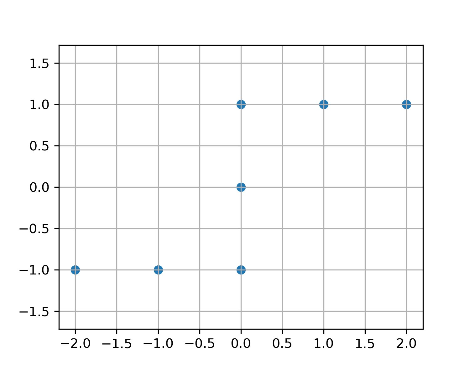
Find the weight vectors for the data matrix \(X\) representing the points:

Solution

\[\begin{split} \boldsymbol{w}_1 = \frac{1}{2 \sqrt{20 - 2 \sqrt{10}}} \begin{bmatrix} 6 \\ 2(\sqrt{10} - 1) \end{bmatrix} \end{split}\]

\[\begin{split} \boldsymbol{w}_2 = \frac{1}{2 \sqrt{20 - 2 \sqrt{10}}} \begin{bmatrix} 2(\sqrt{10} - 1) \\ -6 \end{bmatrix} \end{split}\]

Suppose \(X\) is a \(100 \times 4\) data matrix such that

\[\begin{split} X^T X = \begin{bmatrix} 2 & 0 & 0 & 0 \\ 0 & 1.5 & 0 & 0 \\ 0 & 0 & 2 & 1 \\ 0 & 0 & 1 & 2 \end{bmatrix} \end{split}\]

Find all the weight vectors of \(X\).

Suppose we want to solve a system \(A \boldsymbol{x} = \boldsymbol{b}\). A small change \(\Delta \boldsymbol{b}\) produces a change in the solution

\[ A(\boldsymbol{x} + \Delta \boldsymbol{x}) = \boldsymbol{b} + \Delta \boldsymbol{b} \]

Describe the unit vector \(\Delta \boldsymbol{b}\) that will produce the largest change \(\| \Delta \boldsymbol{x} \|\).

Find the rank 2 pseudo inverse

\[ A_2^+ = \frac{1}{\sigma_1} \boldsymbol{q}_1 \boldsymbol{p}_1^T + \frac{1}{\sigma_2} \boldsymbol{q}_2 \boldsymbol{p}_2^T \]

of the matrix

\[\begin{split} A = \left[ \begin{array}{rrr} 1 & 1 & 1 \\ 1 & 0 & -2 \\ 1 & -1 & 1 \end{array} \right] \end{split}\]

(Note: the columns of \(A\) are orthogonal.)

Let \(A\) be a \(m \times n\) matrix with singular value decomposition \(A = P \Sigma Q^T\). Let \(k < \min\{m,n\}\) and let

\[ A_k = \sum_{i=1}^k \sigma_i \boldsymbol{p}_i \boldsymbol{q}_i^T \]

Describe the singular value decomposition of \(A - A_k\).