Deblurring Images

import numpy as np
import scipy.linalg as la
import matplotlib.pyplot as plt
from scipy.io import loadmat

plt.set_cmap('binary')

<Figure size 640x480 with 0 Axes>

Blurring images by Toeplitz matrices

Represent a image as a matrix \(X\). Use the function scipy.linalg.toeplitz to create a Toeplitz matrices \(A_c\) and \(A_r\). Matrix multiplication on the left \(A_c X\) blurs vertically (in the columns) and on the right \(X A_r\) blurs horizontally (in the rows).

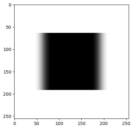
Let us create a \(N \times N\) matrix of zeros and ones such that represents the image of square.

N = 256

Z = np.zeros((N//4,N//4))
O = np.ones((N//4,N//4))
X = np.block([[Z,Z,Z,Z],[Z,O,O,Z],[Z,O,O,Z],[Z,Z,Z,Z]])
plt.imshow(X)
plt.show()

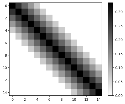
Create a Toeplitz matrix where the values decrease linearly from the diagonal.

c = np.zeros(N)
s = 5
c[:s] = (s - np.arange(0,s))/(3*s)
Ac = la.toeplitz(c)

plt.imshow(Ac[:15,:15])
plt.colorbar()
plt.show()

Check the condition number of \(A_c\).

np.linalg.cond(Ac)

24782.331042560716

Blur the image \(X\) vertically.

plt.imshow(Ac @ X)
plt.show()

Do the same but in the horizontal direction.

r = np.zeros(N)
s = 20
r[:s] = (s - np.arange(0,s))/(3*s)
Ar = la.toeplitz(r)

plt.imshow(X @ Ar.T)
plt.show()

Combine both vertical and horizontal blurring.

plt.imshow(Ac @ X @ Ar.T)
plt.show()

Inverting the noise

Let \(E\) represent some noise in the recording of the image

\[ A_c X A_r^T = B + E \]

How do we find \(X\)?

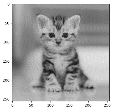
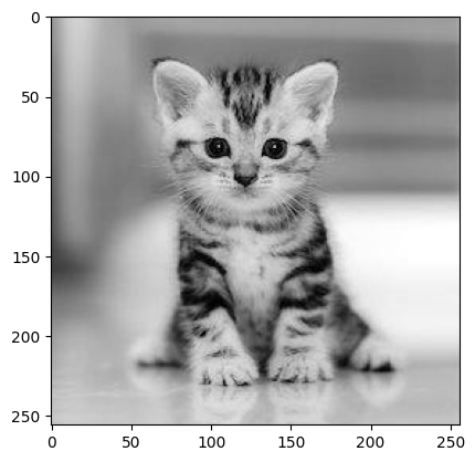
kitten = plt.imread('data/kitten.jpg').astype(np.float64)

kitten.shape

(256, 256)

plt.imshow(kitten,cmap='gray')
plt.show()

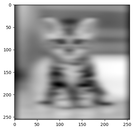
B = Ac@kitten@Ar.T + 0.01*np.random.randn(256,256)

plt.imshow(B,cmap='gray')
plt.show()

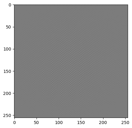
X1 = la.solve(Ac,B)
X2 = la.solve(Ar,X1.T)
X2 = X2.T

plt.imshow(X2,cmap='gray')
plt.show()

Truncated SVD

We need to avoid inverting the noise therefore we compute using the truncated pseudoinverse

\[ X = (A_c)_k^+ B (A_r^T)_k^+ \]

Pc,Sc,QTc = la.svd(Ac)

Pr,Sr,QTr = la.svd(Ar)

k = 200
Dc_k_plus = np.hstack([1/Sc[:k],np.zeros(N-k)])
Dr_k_plus = np.hstack([1/Sr[:k],np.zeros(N-k)])
Ac_k_plus = QTc.T @ np.diag(Dc_k_plus) @ Pc.T
Ar_k_plus = Pr @ np.diag(Dr_k_plus) @ QTr
X = Ac_k_plus @ B @ Ar_k_plus
plt.imshow(X,cmap='gray')
plt.show()