Least Squares Approximation

Find the least squares approximation of the system \(A \boldsymbol{x} \approx \boldsymbol{b}\) by minimizing the distance \(\| A \boldsymbol{x} - \boldsymbol{b}\|\). There are several methods to find the approximation including the normal equations and the QR equations.

Definition

Let \(A\) be an \(m \times n\) matrix with \(m > n\) and \(\mathrm{rank}(A) = n\). The least squares approximation of the system \(A \boldsymbol{x} \approx \boldsymbol{b}\) is the vector \(\boldsymbol{x}\) which minimizes the distance \(\| A\boldsymbol{x} - \boldsymbol{b} \|\).

Normal Equations

Let \(A\) be an \(m \times n\) matrix with \(m > n\) and \(\mathrm{rank}(A) = n\). The least squares approximation of the system \(A \boldsymbol{x} \approx \boldsymbol{b}\) is the solution of the system

\[ A^TA\boldsymbol{x} = A^T\boldsymbol{b} \]

The system is called the normal equations.

Proof

If \(\boldsymbol{x} \in \mathbb{R}^n\), then \(A \boldsymbol{x} \in R(A)\). The projection theorem states that the point in \(R(A)\) nearest to \(\boldsymbol{b} \in \mathbb{R}^m\) is the orthogonal projection of \(\boldsymbol{b}\) onto \(R(A)\). If \(\boldsymbol{x}\) is the vector such that \(A\boldsymbol{x} = \mathrm{proj}_{R(A)}(\boldsymbol{b})\), then \(A\boldsymbol{x} - \boldsymbol{b}\) is in \(R(A)^{\perp}\) and therefore

\[ A^T(A\boldsymbol{x} - \boldsymbol{b}) = 0 \ \ \Rightarrow \ \ A^TA\boldsymbol{x} = A^T\boldsymbol{b} \]

We assume \(\mathrm{rank}(A) = n\), therefore \(A^TA\) is nonsingular and the solution exists and is unique.

QR Equations

Let \(A\) be an \(m \times n\) matrix with \(m > n\) and \(\mathrm{rank}(A) = n\). The least squares approximation of the system \(A \boldsymbol{x} \approx \boldsymbol{b}\) is the solution of the system of equations

\[ R_1\boldsymbol{x} = Q_1^T \boldsymbol{b} \]

where \(A = Q_1 R_1\) is the thin QR decomopsition. The system is called the QR equations. Futhermore, the residual is given by

\[ \| A \boldsymbol{x} - \boldsymbol{b} \| = \| Q_2^T \boldsymbol{b} \| \]

where \(A = QR\) is the QR deomposition with \(Q = [ Q_1 \ \ Q_2 ]\).

Proof

The matrix \(Q\) is orthogonal therefore

\[ \| A \boldsymbol{x} - \boldsymbol{b} \|^2 = \| Q(R \boldsymbol{x} - Q^T\boldsymbol{b}) \|^2 = \| R \boldsymbol{x} - Q^T\boldsymbol{b} \|^2 \]

\[\begin{split} = \left\| \begin{bmatrix} R_1 \\ \boldsymbol{0} \end{bmatrix} \boldsymbol{x} - \begin{bmatrix} Q_1^T \\ Q_2^T \end{bmatrix} \boldsymbol{b} \right\|^2 = \left\| \begin{bmatrix} R_1 \boldsymbol{x} \\ \boldsymbol{0} \end{bmatrix} - \begin{bmatrix} Q_1^T \boldsymbol{b} \\ Q_2^T \boldsymbol{b} \end{bmatrix} \right\|^2 \end{split}\]

\[\begin{split} = \left\| \begin{bmatrix} R_1 \boldsymbol{x} - Q_1^T \boldsymbol{b} \\ -Q_2^T \boldsymbol{b} \end{bmatrix} \right\|^2 = \| R_1 \boldsymbol{x} - Q_1^T \boldsymbol{b} \|^2 + \| Q_2^T \boldsymbol{b} \|^2 \end{split}\]

where we use the Pythagoras theorem in the last equality. The vector \(Q_2^T \boldsymbol{b}\) does not depend on \(\boldsymbol{x}\) therefore the minimum value of \(\| A \boldsymbol{x} - \boldsymbol{b} \|\) occurs when \(R_1 \boldsymbol{x} = Q_1^T \boldsymbol{b}\) and the residual is \(\| A \boldsymbol{x} - \boldsymbol{b} \| = \| Q_2^T \boldsymbol{b} \|\).

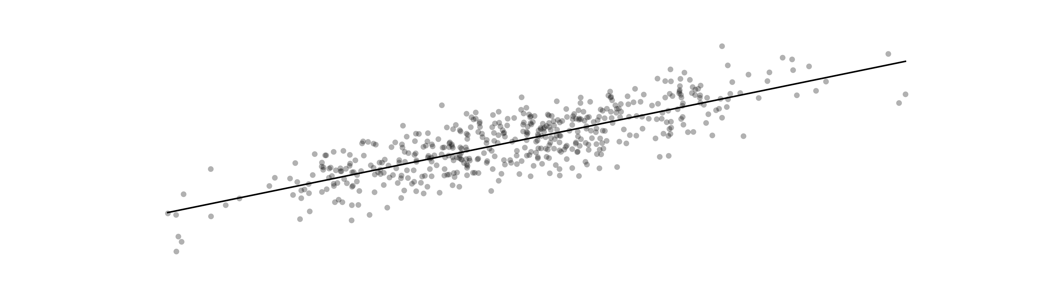
Fitting Models to Data

Suppose we have \(m\) points

\[ (t_1,y_1) , \dots , (t_m,y_m) \]

and we want to find a line

\[ y=c_1 + c_2t \]

that “best fits” the data. There are different ways to quantify what “best fits” means but the most common method is called least squares linear regression. In least squares linear regression, we want to minimize the sum of squared errors

\[ SSE = \sum_i (y_i - (c_1 + c_2 t_i))^2 \]

In matrix notation, the sum of squared errors is

\[ SSE = \Vert \boldsymbol{y} - A \boldsymbol{c} \Vert^2 \]

where

\[\begin{split} \boldsymbol{y} = \begin{bmatrix} y_1 \\ y_2 \\ \vdots \\ y_m \end{bmatrix} \hspace{10mm} A = \begin{bmatrix} 1 & t_1 \\ 1 & t_2 \\ \vdots & \vdots \\ 1 & t_m \end{bmatrix} \hspace{10mm} \boldsymbol{c} = \begin{bmatrix} c_1 \\ c_2 \end{bmatrix} \end{split}\]

We assume that \(m \geq 2\) and \(t_i \not= t_j\) for all \(i \not= j\) which implies \(\mathrm{rank}(A) = 2\). Therefore the vector of coefficients

\[\begin{split} \boldsymbol{c} = \begin{bmatrix} c_1 \\ c_2 \end{bmatrix} \end{split}\]

is the least squares approximation of the system \(A \boldsymbol{c} \approx \boldsymbol{y}\). See Wikipedia:Simple linear regression.

More generally, given \(m\) data points

\[ (t_1,y_1) , \dots , (t_m,y_m) \]

and a model function \(f(t,\boldsymbol{c})\) which depends on parameters \(c_1,\dots,c_n\), the least squares data fitting problem consists of computing parameters \(c_1,\dots,c_n\) which minimize the sum of squared errors

\[ SSE = \sum_i (y_i - f(t_i,\boldsymbol{c}))^2 \]

If the model function is of the form

\[ f(t,\boldsymbol{c}) = c_1 f_1(t) + \cdots + c_n f_n(t) \]

for some functions \(f_1(t),\dots,f_n(t)\) then we say the data fitting problem is linear (but note the function \(f_1,\dots,f_n\) are not necessarily linear). In the linear case, use matrix notation to write the sum of squared errors as

\[ SSE = \Vert \boldsymbol{y} - A \boldsymbol{c} \Vert^2 \]

where

\[\begin{split} \boldsymbol{y} = \begin{bmatrix} y_1 \\ y_2 \\ \vdots \\ y_m \end{bmatrix} \hspace{10mm} A = \begin{bmatrix} f_1(t_1) & f_2(t_1) & \cdots & f_n(t_1) \\ f_1(t_2) & f_2(t_2) & \cdots & f_n(t_2) \\ \vdots & \vdots & \ddots & \vdots \\ f_1(t_m) & f_2(t_m) & \cdots & f_n(t_m) \end{bmatrix} \hspace{10mm} \boldsymbol{c} = \begin{bmatrix} c_1 \\ c_2 \\ \vdots \\ c_n \end{bmatrix} \end{split}\]

We assume that \(m \geq n\) and \(f_1,\dots,f_n\) are linearly independently (which implies \(\mathrm{rank}(A) = n\)). Therefore the vector of coefficients \(\boldsymbol{c}\) is the least squares approximation of the system \(A \boldsymbol{c} \approx \boldsymbol{y}\).

Exercises

Let \(A = QR\) where

\[\begin{split} Q = \left[ \begin{array}{rrrrr} 0 & 0 & 0 & 1 & 0 \\ 0 & 1 & 0 & 0 & 0 \\ 0 & 0 & 1 & 0 & 0 \\ 1 & 0 & 0 & 0 & 0 \\ 0 & 0 & 0 & 0 & 1 \end{array} \right] \ \ R = \left[ \begin{array}{rrrr} 1 & 1 & 1 & 1 \\ 0 & 1 & 1 & 1 \\ 0 & 0 & 1 & 1 \\ 0 & 0 & 0 & 1 \\ 0 & 0 & 0 & 0 \end{array} \right] \end{split}\]

Find the least squares approximation \(A\boldsymbol{x} \approx \boldsymbol{b}\) where

\[\begin{split} \boldsymbol{b} = \left[ \begin{array}{r} -2 \\ -1 \\ 0 \\ 1 \\ 2 \end{array} \right] \end{split}\]

Solution

\[\begin{split} \boldsymbol{x} = \left[ \begin{array}{r} 2 \\ -1 \\ 2 \\ -2 \end{array} \right] \end{split}\]

Setup (but do not solve) a linear system \(A \boldsymbol{c} = \boldsymbol{y}\) where the solution is the coefficient vector

\[\begin{split} \boldsymbol{c} = \begin{bmatrix} c_0 \\ c_1 \\ c_2 \end{bmatrix} \end{split}\]

such that the function

\[ f(t) = c_0 + c_1\cos(2 \pi t) + c_2 \sin(2 \pi t) \]

bests fits the data \((0,1),(1/4,3),(1/2,2),(3/4,-1),(1,0)\).

Solution

\[\begin{split} A = \left[ \begin{array}{rrr} 1 & 1 & 0 \\ 1 & 0 & 1 \\ 1 & -1 & 0 \\ 1 & 0 & -1 \\ 1 & 1 & 0 \end{array} \right] \hspace{10mm} \boldsymbol{y} = \left[ \begin{array}{r} 1 \\ 3 \\ 2 \\ -1 \\ 0 \end{array} \right] \end{split}\]