Fitting Models to Data

import numpy as np
import matplotlib.pyplot as plt
import scipy.linalg as la

Linear Regression

Suppose we have \(n+1\) points

\[ (t_0,y_0) , (t_1,y_1) , \dots , (t_n,y_n) \]

and we want to fit a line

\[ y=c_0 + c_1t \]

that “best fits” the data. There are different ways to quantify what “best fit” means but the most common method is called least squares linear regression. In least squares linear regression, we want to minimize the sum of squared errors

\[ SSE = \sum_i (y_i - (c_0 + c_1 t_i))^2 \]

In matrix notation

\[\begin{split} A = \begin{bmatrix} 1 & t_0 \\\ 1 & t_1 \\\ \vdots & \vdots \\\ 1 & t_n \end{bmatrix} \ , \ \ \mathbf{y} = \begin{bmatrix} y_0 \\\ y_1 \\\ \vdots \\\ y_n \end{bmatrix} \ , \ \ \mathbf{c} = \begin{bmatrix} c_0 \\\ c_1 \end{bmatrix} \end{split}\]

then the sum of squared errors can be expressed as

\[ SSE = \Vert \mathbf{y} - A \mathbf{c} \Vert^2 \]

We solve for the coefficients \(\mathbf{c} = [c_0,c_1]^T\) which minimize \(\Vert \mathbf{y} - A \mathbf{c} \Vert^2\) in 2 two ways:

Normal Equations

The coefficient vector \(\mathbf{c}\) is the unique solution of the system

\[ \left( A^T A \right) \mathbf{c} = A^T \mathbf{y} \]

QR Decomposition

Let \(A = Q_1R_1\) be the (thin) QR decomposition of \(A\) (where \(R_1\) is square upper triangular). The coefficient vector \(\mathbf{c}\) is the unique solution of the system

\[ R_1 \mathbf{c} = Q_1^T \mathbf{y} \]

Example: Fake Noisy Linear Data

Let’s do an example with some fake data. Let’s build a set of random points based on the model

\[ y = c_0 + c_1 t + \epsilon \]

for some arbitrary choice of \(c_0\) and \(c_1\). The factor \(\epsilon\) represents some random noise which we model using the normal distribution. We can generate random numbers sampled from the standard normal distribution using the NumPy function numpy.random.randn.

The goal is to demonstrate that we can use linear regression to retrieve the coefficeints \(c_0\) and \(c_1\) from the linear regression calculation.

c0 = 7
c1 = -4
N = 500
t = np.random.rand(N)
noise = 0.3*np.random.randn(N)
y = c0 + c1*t + noise
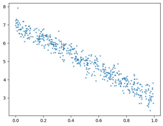
plt.scatter(t,y,alpha=0.7,lw=0,s=10);
plt.show()

Let’s use linear regression to retrieve the coefficients \(c_0\) and \(c_1\). Construct the matrix \(A\):

A = np.column_stack([np.ones(N),t])
print(A.shape)

(500, 2)

Let’s look at the first 5 rows of \(A\) to see that it is in the correct form:

A[:5,:]

array([[1.        , 0.64835034],
       [1.        , 0.19419242],
       [1.        , 0.78607232],
       [1.        , 0.51940935],
       [1.        , 0.72293165]])

Use scipy.linalg.solve to solve \(\left(A^T A\right)\mathbf{c} = \left(A^T\right)\mathbf{y}\) for \(\mathbf{c}\):

c = la.solve(A.T @ A, A.T @ y)
print(c)

[ 7.02789431 -4.03227316]

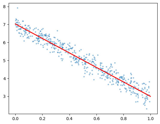
We have retrieved the coefficients of the model almost exactly! Let’s plot the random data points with the linear regression we just computed.

ts = np.linspace(0,1,10)
ys = c[0] + c[1]*ts
plt.plot(ts,ys,'r',linewidth=2)
plt.scatter(t,y,alpha=0.5,lw=0,s=10);
plt.show()

Polynomial Regression

The same idea works for fitting a degree \(d\) polynomial model

\[ y = c_0 + c_1t + c_2t^2 + \cdots + c_dt^d \]

to a set of \(n+1\) data points

\[ (t_0,y_0), (t_1,y_1), \dots , (t_n,y_n) \]

We form the matrices as before but now the Vandermonde matrix \(A\) has \(d+1\) columns

\[\begin{split} A = \begin{bmatrix} 1 & t_0 & t_0^2 & \cdots & t_0^d \\\ 1 & t_1 & t_1^2 & \cdots & t_1^d \\\ & \vdots & & & \vdots \\\ 1 & t_n & t_n^2 & \cdots & t_n^d \end{bmatrix} \ , \ \ \mathbf{y} = \begin{bmatrix} y_0 \\\ y_1 \\\ \vdots \\\ y_n \end{bmatrix} \ , \ \ \mathbf{c} = \begin{bmatrix} c_0 \\\ c_1 \\\ c_2 \\\ \vdots \\\ cd_d \end{bmatrix} \end{split}\]

The coefficients \(\mathbf{c} = [c_0,c_1,c_2,\dots,c_d]^T\) which minimize the sum of squared errors \(SSE\) is the unique solution of the linear system

\[ \left( A^T A \right) \mathbf{c} = \left( A^T \right) \mathbf{y} \]

Example: Fake Noisy Quadratic Data

Let’s build some fake data using a quadratic model \(y = c_0 + c_1x + c_2x^2 + \epsilon\) and use linear regression to retrieve the coefficients \(c_0\), \(c_1\) and \(c_2\).

c0 = 3
c1 = 5
c2 = 8
N = 1000
t = 2*np.random.rand(N) - 1 # Random numbers in the interval (-1,1)
noise = np.random.randn(N)
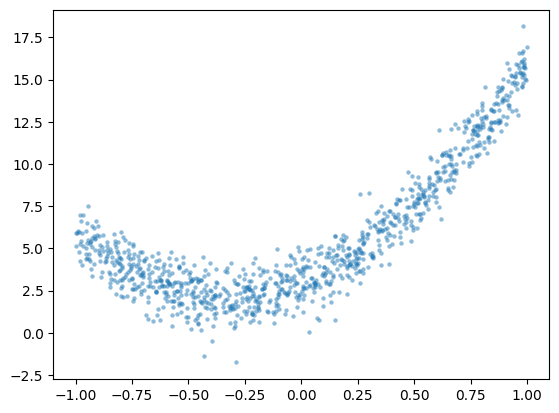
y = c0 + c1*t + c2*t**2 + noise
plt.scatter(t,y,alpha=0.5,lw=0,s=10);
plt.show()

Construct the matrix \(A\):

A = np.column_stack([np.ones(N),t,t**2])

Use scipy.linalg.solve to solve \(\left( A^T A \right) \mathbf{c} = \left( A^T \right) \mathbf{y}\):

c = la.solve(A.T @ A,A.T @ y)

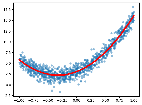
Plot the result:

ts = np.linspace(-1,1,20)
ys = c[0] + c[1]*ts + c[2]*ts**2
plt.plot(ts,ys,'r',linewidth=4)
plt.scatter(t,y,alpha=0.5,lw=0)
plt.show()

Let’s solve again but this time we use the QR decomposition:

Q1,R1 = la.qr(A,mode='economic')
b = Q1.T @ y
c1 = la.solve(R1,b[:3])

Plot the result:

ts = np.linspace(-1,1,20)
ys = c1[0] + c1[1]*ts + c1[2]*ts**2
plt.plot(ts,ys,'r',linewidth=4)
plt.scatter(t,y,alpha=0.5,lw=0)
plt.show()