Differential Equations

Differential Equations#

Most differential equations are impossible to solve exactly and so we use numerical methods such as the finite difference method to approximate solutions. The finite difference method applied to a linear differential equation yields a linear system of equations \(A \boldsymbol{y} = \boldsymbol{b}\).

Second Order Differential Equations#

An ordinary differential equation is an equation involving an unknown function \(y(t)\) and its derivatives. The order of a differential equation is the highest order derivative appearing in the equation. There are many kinds of differential equations. In this section, we consider only second order linear ordinary differential equations

\[ y'' + p(t)y' + q(t)y = r(t) \]

Boundary conditions are equations imposed on the solution at the boundary points \(t_0\) and \(t_f\). For example, specify values of the solution \(y(t)\) at the endpoints

\[ y(t_0) = \alpha \hspace{5mm} y(t_f) = \beta \]

or specify a value of the solution \(y(t)\) at one endpoint and a value of the derivative \(y'(t)\) at the other endpoint

\[ y'(t_0) = \alpha \hspace{5mm} y(t_f) = \beta \]

See Wikipedia:Differential equation.

Finite Difference Method#

The Taylor series of a smooth function \(f(x)\) centered at \(x=a\) is

\[ f(x) = \sum_{n=0}^{\infty} \frac{f^{(n)}(a)}{n!} (x-a)^n = f(a) + f'(a)(x-a) + \frac{f''(a)}{2}(x-a)^2 + \frac{f'''(a)}{6}(x-a)^3 + \cdots \]

See Wikipedia:Taylor series.

Finite difference formulas are derived from Taylor series. Let \(y(t)\) be a smooth function and consider the Taylor series

\[\begin{split} \begin{align*} y(t+h) &= y(t) + y'(t)h + \frac{y''(t)}{2}h^2 + \cdots \\ y(t-h) &= y(t) - y'(t)h + \frac{y''(t)}{2}h^2 + \cdots \end{align*} \end{split}\]

Truncate and rearrange the first series for the forward difference formula

\[ y'(t) \approx \frac{y(t+h) - y(t)}{h} \]

Truncate and rearrange the second series for the backward difference formula

\[ y'(t) \approx \frac{y(t) - y(t - h)}{h} \]

Subtract \(y(t+h) - y(t-h)\) and truncate to get the (first order) central difference formula

\[ y'(t) \approx \frac{y(t+h) - y(t-h)}{2h} \]

Add \(y(t+h) + y(t-h)\) and truncate to get the (second order) central difference formula

\[ y''(t) \approx \frac{y(t+h) -2y(t) + y(t-h)}{h^2} \]

See Wikipedia:Finite difference.

The finite difference method applied to a second order linear ordinary differential equation with boundary conditions

\[ y'' + p(t)y' + q(t)y = r(t) \ \ , \ \ t \in [t_0,t_f] \]

Discretize the domain: choose \(N\), let \(\displaystyle h = \frac{t_f - t_0}{N+1}\) and define \(t_k = t_0 + kh\).
Let \(y_k \approx y(t_k)\) denote the approximation of the solution at \(t_k\).
Substitute finite difference formulas into the equation to define an equation at each \(t_k\).
Rearrange the system of equations into a linear system \(A \boldsymbol{y} = \boldsymbol{b}\) and solve for

\[\begin{split} \boldsymbol{y} = \begin{bmatrix} y_1 \\ y_2 \\ \vdots \\ y_N \end{bmatrix} \end{split}\]

Consider a second order linear ordinary differential equation with boundary conditions of the form

\[ y'' = r(t) \ \ , \ \ y(t_0) = \alpha \ , \ \ y(t_f) = \beta \]

Choose \(N\) and let \(\displaystyle h = (t_f - t_0)/(N+1)\) and define \(t_k = t_0 + kh\). Let \(y_k\) denote an approximation of \(y(t_k)\). Note that the boundary conditions give us \(y_0 = \alpha\) and \(y_{N+1} = \beta\) and let

\[\begin{split} \boldsymbol{y} = \begin{bmatrix} y_1 \\ y_2 \\ \vdots \\ y_N \end{bmatrix} \end{split}\]

Let \(r_k = r(t_k)\) and substitute the central difference formula at \(t_k\) into the differential equation

\[ \frac{y_{k+1} -2y_k + y_{k-1}}{h^2} = r_k \]

Therefore we have \(N\) equations and \(N\) unknowns \(y_k\) for \(k=1,\dots,N\). Use the boundary conditions \(y_0 = \alpha\) and \(y_{N+1} = \beta\) and rearrange the equations

\[\begin{split} \begin{array}{rrrrrrcrrrrcc} - 2y_1 & + & y_2 & & & & & & & & & = & h^2 r_1 - \alpha \\ y_1 & - & 2y_2 & + & y_3 & & & & & & & = & h^2 r_2 \\ & & y_2 & - & 2y_3 & + & y_4 & & & & & = & h^2 r_3 \\ & & & & & & \ddots & & & & & \vdots & \\ & & & & & & y_{N-2} & - & 2y_{N-1} & + & y_N & = & h^2 r_{N-1} \\ & & & & & & & & y_{N-1} & - & 2y_N & = & h^2 r_N - \beta \end{array} \end{split}\]

Rewrite in matrix form \(A \boldsymbol{y} = \boldsymbol{b}\) where

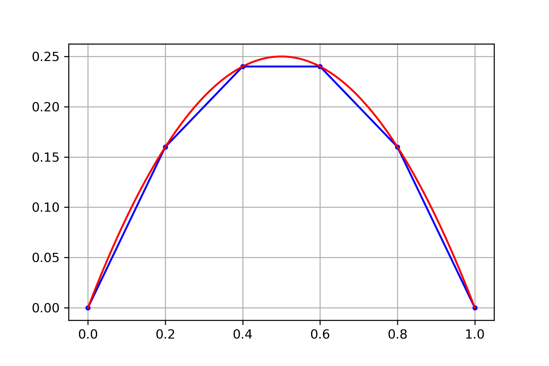
\[\begin{split} A = \left[ \begin{array}{rrcrr} -2 & 1 & & & \\ 1 & -2 & 1 & & \\ & & \ddots & & \\ & & 1 & -2 & 1 \\ & & & 1 & -2 \end{array} \right] \hspace{10mm} \boldsymbol{b} = \begin{bmatrix} h^2 r_1 - \alpha \\ h^2 r_2 \\ \vdots \\ h^2 r_{N-1} \\ h^2 r_N - \beta \end{bmatrix} \end{split}\]

Setup a linear system \(A \boldsymbol{y} = \boldsymbol{b}\) for the equation with boundary conditions

\[ y'' = -2 \ \ , \ \ y(0) = 0 \ , \ \ y(1) = 0 \]

using step size \(h=0.2\).

The step size \(h\) corresponds to \(N=4\) in our formulation, and \(r(t) = -2\), \(\alpha = \beta = 0\) therefore

\[\begin{split} \left[ \begin{array}{rrrr} -2 & 1 & & \\ 1 & -2 & 1 & \\ & 1 & -2 & 1 \\ & & 1 & -2 \end{array} \right] \begin{bmatrix} y_1 \\ y_2 \\ y_3 \\ y_4 \end{bmatrix} = \begin{bmatrix} -0.08 \\ -0.08 \\ -0.08 \\ -0.08 \end{bmatrix} \end{split}\]

Solve the system to find

\[\begin{split} \begin{bmatrix} y_1 \\ y_2 \\ y_3 \\ y_4 \end{bmatrix} = \begin{bmatrix} 0.16 \\ 0.24 \\ 0.24 \\ 0.16 \end{bmatrix} \end{split}\]

The equation is very simple and we can solve exactly by integrating twice

\[ y(t) = -t^2 + C_1t + C_2 \]

The boundary conditions imply \(C_1 = 1\) and \(C_2 = 0\) and therefore the exact solution is

\[ y(t) = t - t^2 \]

Notice that our finite difference approximation found the exact values \(y(0.2) = 0.16\), \(y(0.4) = 0.24\), \(y(0.6) = 0.24\), \(y(0.8) = 0.16\). This is because our equation is very simple and the solution is a polynomial of degree 2. The finite difference method does not compute exact values in general.

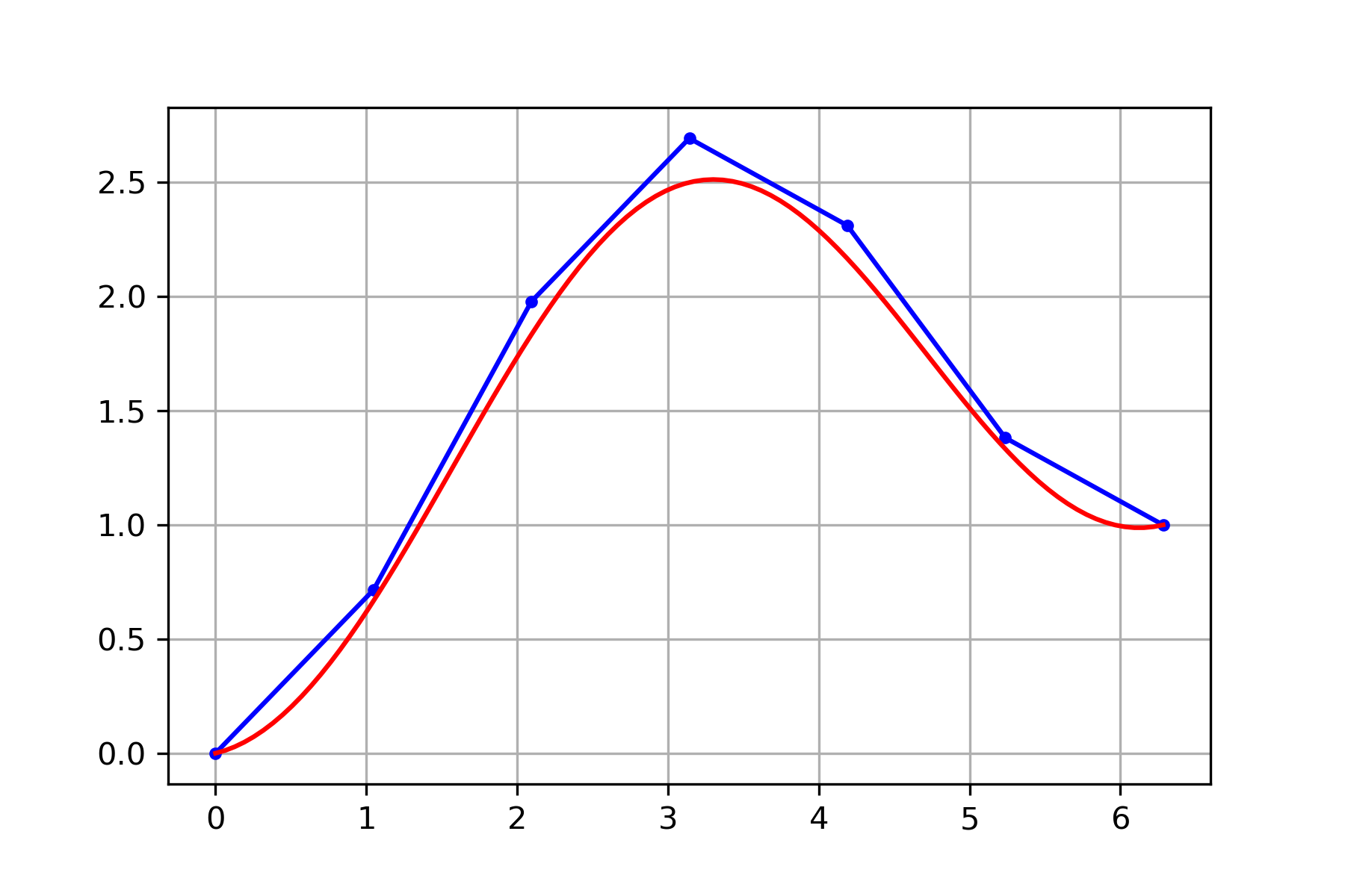
Setup a linear system \(A \boldsymbol{y} = \boldsymbol{b}\) for the equation with boundary conditions

\[ y'' = \cos(t) \ \ , \ \ y(0) = 0 \ , \ \ y(2\pi) = 1 \]

using 7 equally spaced points from \(t_0 = 0\) to \(t_f = 2\pi\).

The value \(N=5\) corresponds to 7 equally spaced points in our formulation with step size

\[ h = \frac{t_f - t_0}{N + 1} = \frac{2\pi - 0}{5 + 1} = \frac{\pi}{3} \]

We have \(r(t) = \cos(t)\) and \(\alpha = 0\) and \(\beta = 1\). Note that \(r_k = \cos(k\pi/3)\) therefore

\[\begin{split} \left[ \begin{array}{rrrrr} -2 & 1 & & & \\ 1 & -2 & 1 & & \\ & 1 & -2 & 1 & \\ & & 1 & -2 & 1 \\ & & & 1 & -2 \end{array} \right] \begin{bmatrix} y_1 \\ y_2 \\ y_3 \\ y_4 \\ y_5 \end{bmatrix} = \begin{bmatrix} \pi^2/18 \\ -\pi^2/18 \\ -\pi^2/9 \\ -\pi^2/18 \\ \pi^2/18 - 1 \end{bmatrix} \end{split}\]

Use scipy.linalg.solve to compute the solution. The equation is elementary and we can solve exactly by integrating twice

\[ y(t) = 1 - \cos(t) + \frac{t}{2 \pi} \]

Plot the exact solution together with our approximation

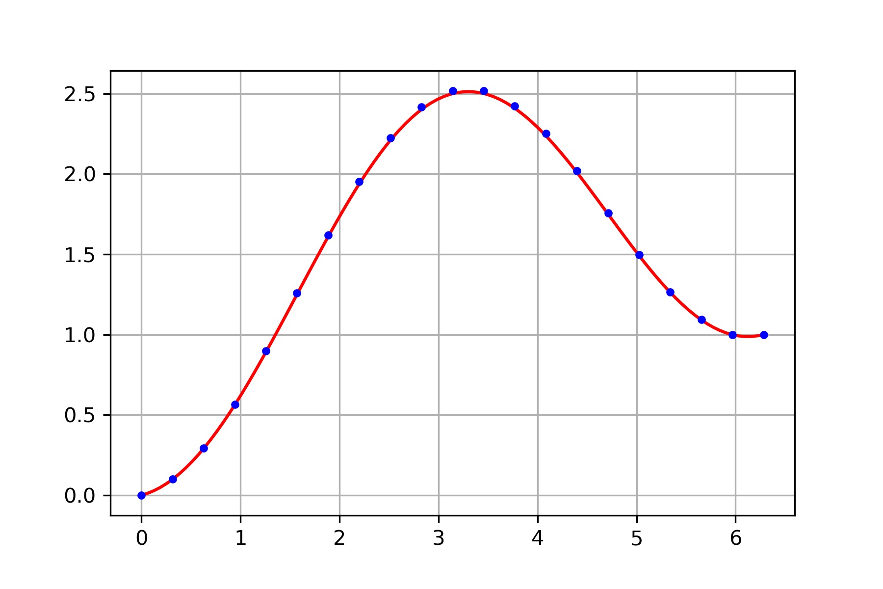
Increasing the number of points in the discretization (equivalently, decreasing the step size \(h\)) decreases the error but increases the number of computations. This is a general principle in numerical computing: higher accuracy requires more computations. For example, consider the same equation as the previous example

\[ y'' = \cos(t) \ \ , \ \ y(0) = 0 \ , \ \ y(2\pi) = 1 \]

but now use 21 equally spaced points from \(t_0 = 0\) to \(t_f = 2\pi\). Then \(N=19\) and

\[ h = \frac{t_f - t_0}{N + 1} = \frac{2\pi - 0}{19 + 1} = \frac{\pi}{10} \]

and the finite difference method produces a much better solution

Consider the general form of a second order linear ordinary differential equation with boundary conditions

\[ y'' + p(t)y' + q(t)y = r(t) \ \ , \ \ y(t_0) = \alpha \ , \ \ y(t_f) = \beta \]

Choose \(N\) and let \(\displaystyle h = \frac{t_f - t_0}{N+1}\) and define \(t_k = t_0 + kh\). Let \(y_k\) denote an approximation of \(y(t_k)\). Note that the boundary conditions give us \(y_0 = \alpha\) and \(y_{N+1} = \beta\) and let

\[\begin{split} \boldsymbol{y} = \begin{bmatrix} y_1 \\ y_2 \\ \vdots \\ y_N \end{bmatrix} \end{split}\]

Let \(p_k = p(t_k)\), \(q_k = q(t_k)\) and \(r_k = r(t_k)\), and substitute the central difference formulas for both \(y''\) and \(y'\) at \(t_k\) into the differential equation

\[ \frac{y_{k+1} -2y_k + y_{k-1}}{h^2} + p_k \frac{y_{k+1} - y_{k-1}}{2h} + q_k y_k = r_k \]

Rearrange the equation

\[\begin{split} \begin{align*} y_{k+1} -2y_k + y_{k-1} + \frac{h p_k}{2} \left( y_{k+1} - y_{k-1} \right) + h^2q_k y_k &= h^2 r_k \\ \left( 1 - \frac{h p_k}{2} \right) y_{k-1} + (h^2q_k - 2)y_k + \left(1 + \frac{h p_k}{2} \right)y_{k+1} &= h^2 r_k \end{align*} \end{split}\]

Introduce the notation

\[ a_k = 1 - \frac{h p_k}{2} \hspace{10mm} b_k = h^2q_k - 2 \hspace{10mm} c_k = 1 + \frac{h p_k}{2} \]

Use the boundary conditions \(y_0 = \alpha\) and \(y_{N+1} = \beta\) and rearrange the equations

\[\begin{split} \begin{array}{rrrrcrrrrcc} b_1 y_1 & + & c_1 y_2 & & & & & & & = & h^2 r_1 - \left( 1 - h p_1/2 \right) \alpha \\ a_2 y_1 & + & b_2 y_2 & + & c_2 y_3 & & & & & = & h^2 r_2 \\ & & & & \ddots & & & & & \vdots & \\ & & & & a_{N-1}y_{N-2} & + & b_{N-1}y_{N-1} & + & c_{N-1}y_N & = & h^2 r_{N-1} \\ & & & & & & a_Ny_{N-1} & + & b_Ny_N & = & h^2 r_N - \left( 1 + h p_N/2 \right) \beta \end{array} \end{split}\]

Rewrite in matrix form \(A \boldsymbol{y} = \boldsymbol{b}\) where

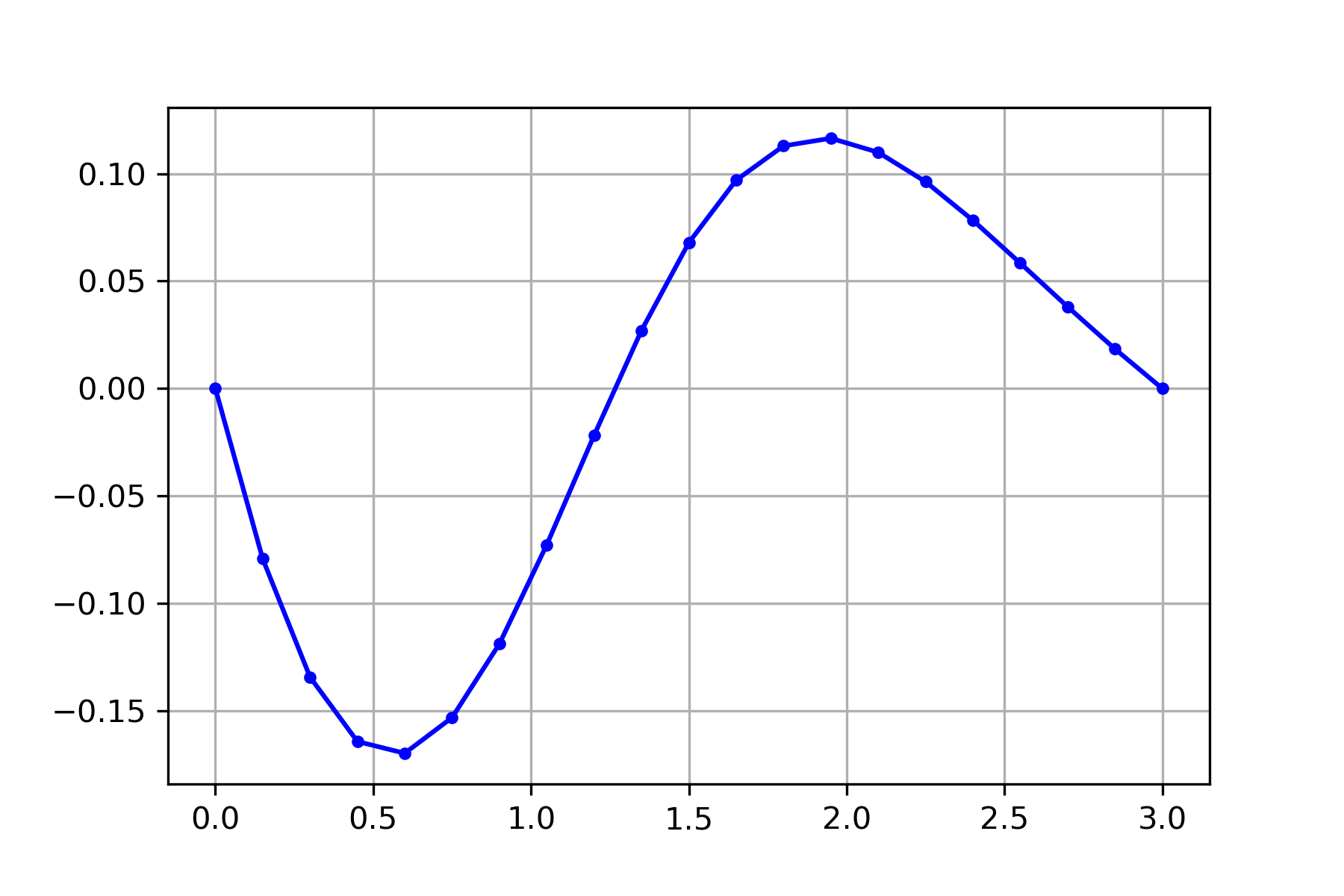
\[\begin{split} A = \left[ \begin{array}{rrcrr} b_1 & c_1 & & & \\ a_2 & b_2 & c_2 & & \\ & & \ddots & & \\ & & a_{N-1} & b_{N-1} & c_{N-1} \\ & & & a_N & b_N \end{array} \right] \hspace{10mm} \boldsymbol{b} = \begin{bmatrix} h^2 r_1 - \left( 1 - h p_1/2 \right) \alpha \\ h^2 r_2 \\ \vdots \\ h^2 r_{N-1} \\ h^2 r_N - \left( 1 + h p_N/2 \right) \beta \end{bmatrix} \end{split}\]

Consider the differential equation with boundary conditions

\[ y'' + t^2y' + y = \cos(t) \ \ , \ \ y(0) = 0 \ , \ \ y(3) = 0 \]

Solving the linear system derived above with \(N=19\) produces the result

Consider a second order linear ordinary differential equation with boundary conditions of the form

\[ y'' = r(t) \ \ , \ \ y'(t_0) = \alpha \ , \ \ y(t_f) = \beta \]

Note that the boundary condition at \(t_0\) specifies the value of the derivative \(y'(t_0) = \alpha\). Use the same notation as in the examples above and apply the central difference formula

\[ y_{k-1} -2y_k + y_{k+1} = h^2 r_k \]

Therefore we have \(N\) equations

\[\begin{split} \begin{array}{rrrrrrcrrrrrrcc} y_0 & - & 2y_1 & + & y_2 & & & & & & & & & = & h^2 r_1 \\ & & y_1 & - & 2y_2 & + & y_3 & & & & & & & = & h^2 r_2 \\ & & & & & & \ddots & & & & & & & \vdots & \\ & & & & & & y_{N-2} & - & 2y_{N-1} & + & y_N & & & = & h^2 r_{N-1} \\ & & & & & & & & y_{N-1} & - & 2y_N & + & y_{N+1} & = & h^2 r_N \end{array} \end{split}\]

We can use \(y_{N+1} = \beta\) and move the term to the right side in the last equation but \(y_0\) in the first equation is unknown. Use the forward difference formula to approximate \(y_0\)

\[ y'(t_0) \approx \frac{y(t_1) - y(t_0)}{h} \ \ \Rightarrow \ \ y_0 = y_1 - h \alpha \]

Therefore we can write the equations in matrix form \(A \boldsymbol{y} = \boldsymbol{b}\) where

\[\begin{split} A = \left[ \begin{array}{rrcrr} -1 & 1 & & & \\ 1 & -2 & 1 & & \\ & & \ddots & & \\ & & 1 & -2 & 1 \\ & & & 1 & -2 \end{array} \right] \hspace{10mm} \boldsymbol{b} = \begin{bmatrix} h^2 r_1 + h\alpha \\ h^2 r_2 \\ \vdots \\ h^2 r_{N-1} \\ h^2 r_N - \beta \end{bmatrix} \end{split}\]

Exercises#

Exercise 1. Determine whether the statement is True or False.

The finite difference method applied to a linear second order differential equation with boundary conditions will compute exact values of the solution \(y_k = y(t_k)\) if the step size \(h\) is chosen to be small enough.
The finite difference method applied to a linear second order differential equation with boundary conditions will never compute exact values of the solution \(y_k = y(t_k)\) for any differential equation and step size \(h\).

Exercise 2. Suppose we discretize the domain \([0,1]\) of a differential equation with boundary conditions

\[ y'' + p(t)y' + q(t)y = r(t) \ \ , \ \ y(0) = \alpha \ \ , \ \ y(1) = \beta \]

with step size \(h=0.1\) and derive a linear system \(A \boldsymbol{y} = \boldsymbol{b}\). How many unknown values \(y_k\) are we solving for in this case?

Exercise 3. Setup a linear system \(A \boldsymbol{y} = \boldsymbol{b}\) to approximate the solution of the equation with boundary conditions

\[ y'' = 2^t \ \ , \ \ y'(0) = 1 \ , \ \ y(1) = 0 \]

using step size \(h=0.25\). Use the forward difference formula and the boundary condition \(y'(0)=1\) to approximate the boundary value \(y_0\).

Exercise 4. Derive the general form of the linear system \(A \boldsymbol{y} = \boldsymbol{b}\) for an equation with boundary conditions

\[ y'' + p(t)y' = r(t) \ \ , \ \ y(t_0) = \alpha \ \ , \ \ y(t_f) = \beta \]

using the forward difference formula to approximate \(y'\). Use the notation as in the examples: choose \(N\), let \(h = (t_f - t_0)/(N+1)\) and \(t_k = t_0 + kh\), let \(y_k\) denote an approximation of \(y(t_k)\) and note \(y_0 = \alpha\) and \(y_{N+1} = \beta\).

Exercise 5. Explain why it is not possible to derive a linear system \(A \boldsymbol{y} = \boldsymbol{b}\) for the equation

\[ y'' = \cos(y) \ \ , \ \ y(0) = 0 \ \ , \ \ y(1) = \frac{\pi}{4} \]

by applying finite difference formulas.

Exercise 6. Suppose we compute the finite difference approximation of the equation

\[ y'' = \frac{5}{1 + t^4} \ \ , \ \ y(0) = 0 \ \ , \ \ y(1) = 1 \]

with 5 equally spaced points from \(t_0 = 0\) to \(t_4 = 1\) and find \(y_1 = -0.19554177\) and \(y_3 = 0.35872678\). Determine \(y_2\).

Exercise 7. Setup a linear system \(A \boldsymbol{y} = \boldsymbol{b}\) for the finite difference approximation of

\[ y'' + ty = 0 \ \ , \ \ y(1) = 1 \ \ , \ \ y(3) = -1 \]

using 5 equally spaced points from \(t_0 = 1\) to \(t_4 = 3\).

Exercise 8. Setup a linear system \(A \boldsymbol{y} = \boldsymbol{b}\) for the finite difference approximation of

\[ y'' + ty = 0 \ \ , \ \ y(1) = 1 \ \ , \ \ y'(3) = -1 \]

using 5 equally spaced points from \(t_0 = 1\) to \(t_4 = 3\). (Hint: use the backwards difference formula to approximate \(y_4\).)

Exercise 9. Setup the linear system \(A \boldsymbol{y} = \boldsymbol{b}\) corresponding to the finite difference method applied to the equation

\[ y'' + y' = t^2 \ \ , \ \ y(-1) = y(1) = 0 \]

using 9 equally spaced points on the domain \([-1,1]\).

Exercise 10. Setup the linear system \(A\boldsymbol{y} = \boldsymbol{b}\) corresponding to the finite difference method applied to the equation

\[ y'' + \cos(t) y = \sin(t) \ \ , \ \ y(0) = y(2\pi) = 0 \]

using 9 equally spaced points on the domain \([0,2\pi]\).

Exercise 11. Setup the linear system \(A\boldsymbol{y} = \boldsymbol{b}\) corresponding to the finite difference method applied to the equation

\[ y'' + \sin(t) y = \cos^2(t) \ \ , \ \ y(0) = y(2\pi) = 0 \]