Linear Systems of Equations

import numpy as np
import scipy.linalg as la
import matplotlib.pyplot as plt

Solve linear systems of equations \(A \mathbf{x} = \mathbf{b}\):

• Create NumPy arrays to represent \(A\) and \(\mathbf{b}\)

• Compute the solution \(\boldsymbol{x}\) using the SciPy function scipy.linalg.solve

Learn about NumPy arrays and the SciPy Linear Algebra package.

Example: Solve \(A \mathbf{x} = \mathbf{b}\) with scipy.linalg.solve

Compute the solution of the system \(A \mathbf{x} = \mathbf{b}\) where

\[\begin{split} A = \begin{bmatrix} 2 & 1 & 1 \\ 2 & 0 & 2 \\ 4 & 3 & 4 \end{bmatrix} \hspace{10mm} \mathbf{b} = \left[ \begin{array}{r} -1 \\ 1 \\ 1 \end{array} \right] \end{split}\]

A = np.array([[2,1,1],[2,0,2],[4,3,4]])
b = np.array([[-1],[1],[1]])

print(A)

[[2 1 1]
 [2 0 2]
 [4 3 4]]

print(b)

[[-1]
 [ 1]
 [ 1]]

type(b)

numpy.ndarray

x = la.solve(A,b)

print(x)

[[-1.16666667]
 [-0.33333333]
 [ 1.66666667]]

Due to rounding errors in the computation, our solution \(\hat{\mathbf{x}}\) is an approximation of the exact solution

\[\begin{split} \mathbf{x} = \left[ \begin{array}{r} -7/6 \\-1/3 \\ 5/3 \end{array} \right] \end{split}\]

Compute the norm of the residual \(\| \mathbf{b} - A \mathbf{x} \|\)

r = la.norm(b - A @ x)

print(r)

2.220446049250313e-16

Example: Resistor Network

Compute the solution of the system \(A \mathbf{x} = \mathbf{b}\) for

\[\begin{split} A = \left[ \begin{array}{cccccccc} 2R & -R & 0 & 0 & \cdots & 0 & 0 & 0 \\ -R & 2R & -R & 0 & & 0 & 0 & 0 \\ 0 & -R & 2R & -R & \cdots & 0 & 0 & 0 \\ \vdots & & \vdots & & \ddots & & \vdots & \\ 0 & 0 & 0 & 0 & \cdots & -R & 2R & -R \\ 0 & 0 & 0 & 0 & \cdots & 0 & -R & 2R \\ \end{array} \right] \hspace{10mm} \mathbf{b} = \left[ \begin{array}{r} V \\ \vdots \\ V \end{array} \right] \end{split}\]

where \(A\) is a square matrix of size \(N\), and \(R\) and \(V\) are some positive constants. The system is a mathematical model of the parallel circuilt

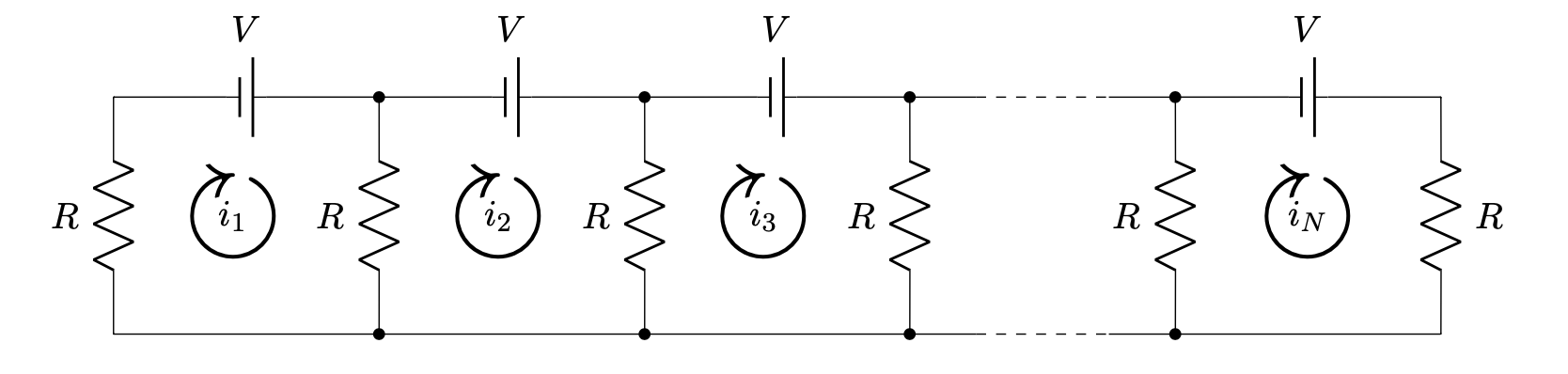
such that the solution consists of the loops currents \(i_1,\dots,i_N\).

N = 10
R = 1
V = 1
A1 = 2*R*np.eye(N)
A2 = np.diag(-R*np.ones(N-1),1)
A = A1 + A2 + A2.T
b = V*np.ones([N,1])

print(A)

[[ 2. -1.  0.  0.  0.  0.  0.  0.  0.  0.]
 [-1.  2. -1.  0.  0.  0.  0.  0.  0.  0.]
 [ 0. -1.  2. -1.  0.  0.  0.  0.  0.  0.]
 [ 0.  0. -1.  2. -1.  0.  0.  0.  0.  0.]
 [ 0.  0.  0. -1.  2. -1.  0.  0.  0.  0.]
 [ 0.  0.  0.  0. -1.  2. -1.  0.  0.  0.]
 [ 0.  0.  0.  0.  0. -1.  2. -1.  0.  0.]
 [ 0.  0.  0.  0.  0.  0. -1.  2. -1.  0.]
 [ 0.  0.  0.  0.  0.  0.  0. -1.  2. -1.]
 [ 0.  0.  0.  0.  0.  0.  0.  0. -1.  2.]]

print(b)

[[1.]
 [1.]
 [1.]
 [1.]
 [1.]
 [1.]
 [1.]
 [1.]
 [1.]
 [1.]]

x = la.solve(A,b)

plt.plot(x,'b.')
plt.xlabel('Loop current at index i')
plt.ylabel('Loop currents (Amp)')
plt.show()

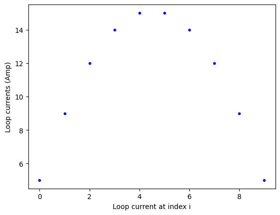
print(x)

[[ 5.]
 [ 9.]
 [12.]
 [14.]
 [15.]
 [15.]
 [14.]
 [12.]
 [ 9.]
 [ 5.]]