Natural Cubic Spline Interpolation

import numpy as np
import scipy.linalg as la
import matplotlib.pyplot as plt
from scipy.interpolate import CubicSpline

Given \(N+1\) data points \((t_0,y_0), \dots , (t_N,y_N)\) we want to construct the natural cubic spline: a piecewise cubic polynomial function \(p(t)\) such that:

• \(p(t)\) is defined by \(N\) cubic polynomials \(p_1(t),p_2(t),\dots,p_N(t)\)

• Each \(p_k(t)\) is defined on the subinterval \([t_{k-1},t_k]\)

• \(p(t)\) is continuous

• \(p(t)\) is smooth (ie. \(p'(t)\) and \(p''(t)\) are continuous)

• \(p(t_k)=y_k\) for all \(k=0,\dots,N\)

Example 1

Consider \((0,0),(1,1),(2,0)\). Construct the linear system for the cubic spline.

A = np.array([[1,1,1,0,0,0],
              [3,2,1,0,0,-1],
              [6,2,0,0,-2,0],
              [0,0,0,1,1,1],
              [0,2,0,0,0,0],
              [0,0,0,6,2,0]])

A

array([[ 1,  1,  1,  0,  0,  0],
       [ 3,  2,  1,  0,  0, -1],
       [ 6,  2,  0,  0, -2,  0],
       [ 0,  0,  0,  1,  1,  1],
       [ 0,  2,  0,  0,  0,  0],
       [ 0,  0,  0,  6,  2,  0]])

y = np.array([1,0,0,-1,0,0]).reshape(6,1)

y

array([[ 1],
       [ 0],
       [ 0],
       [-1],
       [ 0],
       [ 0]])

c = la.solve(A,y)

c

array([[-0.5],
       [ 0. ],
       [ 1.5],
       [ 0.5],
       [-1.5],
       [ 0. ]])

np.linalg.cond(A)

14.530258040767446

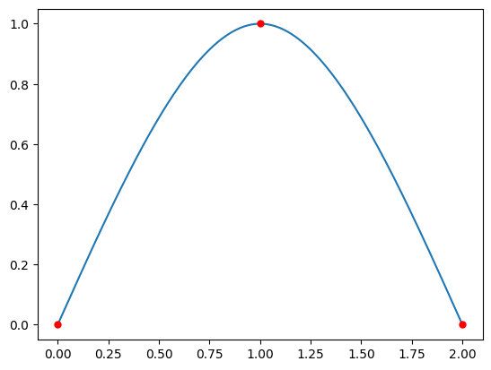
Now let’s use scipy.interpolate.CubicSpline to compute the natural cubic spline and compare our results.

t1 = [0,1,2]
y1 = [0,1,0]
cs1 = CubicSpline(t1,y1,bc_type='natural')
T1 = np.linspace(0,2,200)
Y1 = cs1(T1)
plt.plot(T1,Y1,t1,y1,'r.',markersize=10)
plt.show()

Verify the coefficient matrix:

cs1.c

array([[-0.5,  0.5],
       [ 0. , -1.5],
       [ 1.5,  0. ],
       [ 0. ,  1. ]])

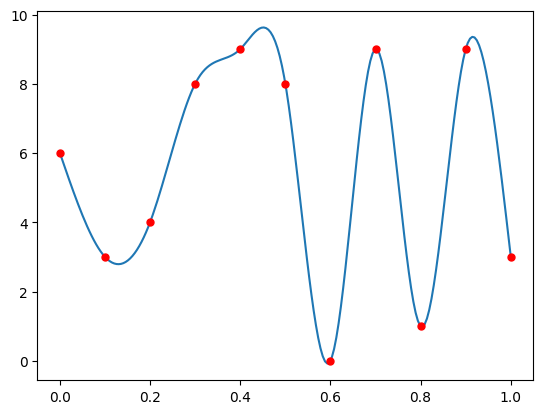
Example 2

N = 10
t2 = np.linspace(0,1,N+1)
y2 = np.random.randint(0,10,N+1)
cs2 = CubicSpline(t2,y2,bc_type='natural')
T2 = np.linspace(0,1,200)
Y2 = cs2(T2)
plt.plot(T2,Y2,t2,y2,'r.',markersize=10)
plt.show()

Example 3

Let’s interpolate the points \(\sin(\pi t_k)\) for \(t_k = k/N\) for \(N=15\) with added noise.

N = 15
t3 = np.linspace(0,1,N+1)
noise = 0.005*np.random.randn(t3.size)
y3 = np.sin(np.pi*t3) + noise
cs3 = CubicSpline(t3,y3)
T3 = np.linspace(0,1,200)
Y3 = cs3(T3)
plt.plot(T3,Y3,'b-',t3,y3,'r.',markersize=10)
plt.grid(True)
plt.show()

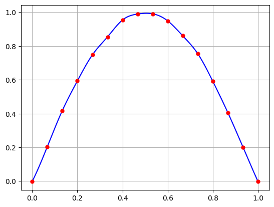
The cubic spline is not sensitive to small changes in the \(y\) values.