Computed Tomography

import numpy as np
import scipy.sparse.linalg as sla
import matplotlib.pyplot as plt
from scipy.io import loadmat

The following example is tomographic X-ray data of a walnut. The dataset was prepared by the Finnish Inverse Problems Society.

data = loadmat('./data/ct.mat')

The data file contains a measurement matrix \(A\) and the projections vector \(m\). These are large matrices and so we need sparse matrices.

Measurement Matrix \(A\)

Each row of the measurement matrix represents a projection of an X-ray through the sample as a particular angle. The measurement matrix is huge! And so we need to use sparse matrices to save memory.

A = data['A']
A.data.nbytes

7762752

A.shape

(9840, 6724)

type(A)

scipy.sparse.csc.csc_matrix

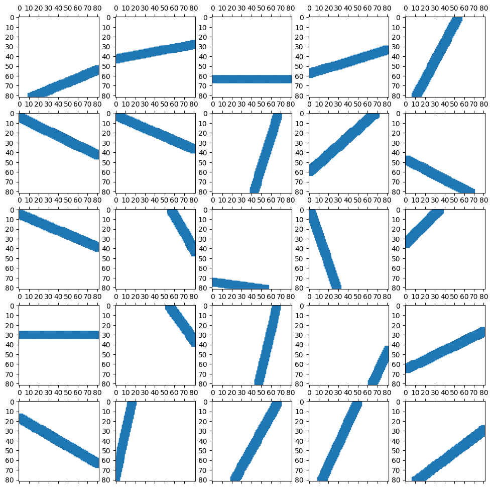
We can visualize each row by reshaping into a matrix. Let’s look at the x-ray projection matrix corresponding to random rows of \(A\).

plt.figure(figsize=(12,12))

N = 5
for i in range(0,N**2):
    plt.subplot(N,N,i+1)
    index = np.random.randint(0,A.shape[0])
    proj = A[index,:].reshape(82,82)
    plt.spy(proj)

plt.show()

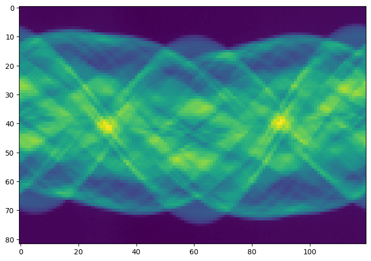
Sinogram: Measured Projections

The vector \(m\) is the collection of 82 projection measurements from 120 different angles.

sinogram = data['m']

sinogram.nbytes

78720

sinogram.shape

(82, 120)

type(sinogram)

numpy.ndarray

plt.figure(figsize=(10,6))
plt.imshow(sinogram)
plt.show()

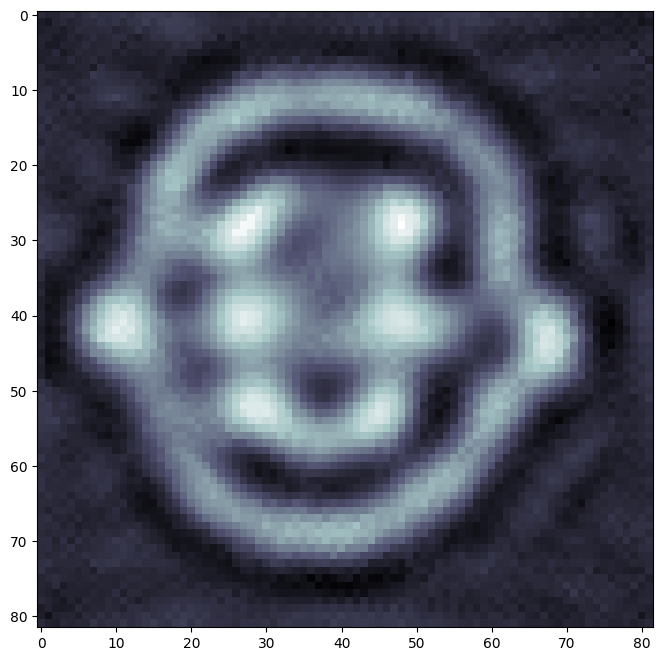
Compute Truncated SVD Solution

We need to solve \(A\mathbf{x} = \mathbf{b}\) (where \(\mathbf{b}\) is the vector of projections) however there are errors in the projections vector \(\mathbf{b}\) and so we actually have

\[ A \hat{\mathbf{x}} = \mathbf{b} + \mathbf{e} \]

where \(\mathbf{e}\) is noise. We need to compute the truncated pseudoinverse to avoid inverting the noise

\[ \hat{\mathbf{x}} = A_k^+ ( \mathbf{b} + \mathbf{e} ) \]

b_e = sinogram.reshape([82*120,1],order='F')

Truncate the measurement matrix after the largest \(k\) singular values and compute the pseudoinverse.

k = 200
P,S,QT = sla.svds(A,k=k)

P.shape

(9840, 200)

QT.shape

(200, 6724)

Compute the rank \(k\) truncated pseudoinverse \(A_k^+\) and \(\hat{\mathbf{x}} = A_k^+ ( \mathbf{b} + \mathbf{e} )\)

A_k_plus = QT.T @ np.diag(1/S) @ P.T
X = A_k_plus @ b_e

Visualize the result by reshaping \(\hat{\mathbf{x}}\) in a square matrix.

plt.figure(figsize=(8,8))
plt.imshow(X.reshape(82,82).T,cmap='bone')
plt.show()

True Solution

Compare to the true solution provided by FIPS.