Principal Component Analysis

import numpy as np
import scipy.linalg as la
from sklearn import datasets
import matplotlib.pyplot as plt

Let \(\mathbf{x}_1,\dots,\mathbf{x}_n \in \mathbb{R}^p\) such that the average of the points is located at the origin

\[ \frac{1}{n} \sum_{k=1}^n \mathbf{x}_k = \mathbf{0} \]

Principal component analysis seeks an orthonormal basis \(\mathbf{w}_1 , \dots , \mathbf{w}_p\) such that \(\mathbf{w}_1\) captures the most information (ie. the most variance of the data), and \(\mathbf{w}_2\) captures the most information orthogonal to \(\mathbf{w}_1\) and so on.

Let \(X\) be the \(n \times p\) data matrix with rows \(\mathbf{x}_1,\dots,\mathbf{x}_n\). The weight vectors \(\mathbf{w}_1 , \dots , \mathbf{w}_p\) are the (right) singular vectors of \(X\). That is, the columns of the matrix \(Q\) in the singular value decomposition \(X = P \Sigma Q^T\).

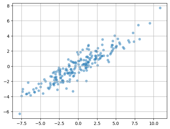
2D Fake Data

N = 200
x = 4*np.random.randn(N)
y = 0.75*np.random.randn(N)
X = np.column_stack((x,y))
X = X - X.mean(axis=0)
theta = np.pi/6
R = np.array([[np.cos(theta),np.sin(theta)],[-np.sin(theta),np.cos(theta)]])
X = X@R
plt.scatter(X[:,0],X[:,1],alpha=0.5,lw=0)
plt.grid(True); plt.axis('equal'); plt.show();

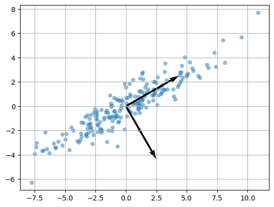
Compute the SVD of the data matrix:

P,S,QT = la.svd(X)

The weight vectors are the rows of \(Q^T\):

QT

array([[ 0.86714106,  0.49806262],
       [ 0.49806262, -0.86714106]])

plt.scatter(X[:,0],X[:,1],alpha=0.5,lw=0)
plt.quiver(QT[0,0],QT[0,1],angles='xy',scale_units='xy',scale=0.2)
plt.quiver(QT[1,0],QT[1,1],angles='xy',scale_units='xy',scale=0.2)
plt.grid(True); plt.axis('equal'); plt.show();

Digits dataset

sklearn is the Python package for machine learning. There are efficient implementations of algorithms such as PCA included in sklearn however let us use the function scipy.linalg.svd.

The digits dataset includes 1797 images of handwritten digits. Let’s import the data.

digits = datasets.load_digits()

D = digits['data']

D.shape

(1797, 64)

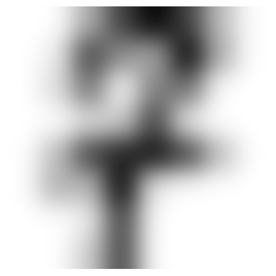
The matrix \(D\) has 1797 rows and 64 columns. Each row is a 8 by 8 pixel image which has been flattened into a row vector of length 64. Select a row, reshape into an 8 by 8 matrix and plot the image.

plt.imshow(D[1056,:].reshape(8,8),cmap='binary',interpolation='gaussian')
plt.axis(False); plt.show();

Normlize the matrix by computing the mean of each column and subtracting the result from every row.

X = D - D.mean(axis=0)

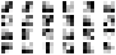
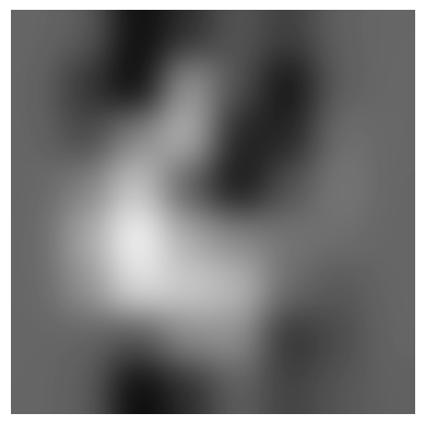
Compute the SVD and plot the first weight vector.

P,S,QT = la.svd(X)

plt.imshow(QT[0,:].reshape(8,8),cmap='binary',interpolation='gaussian')
plt.axis(False); plt.show()

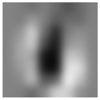
plt.imshow(QT[1,:].reshape(8,8),cmap='binary',interpolation='gaussian')
plt.axis(False); plt.show()

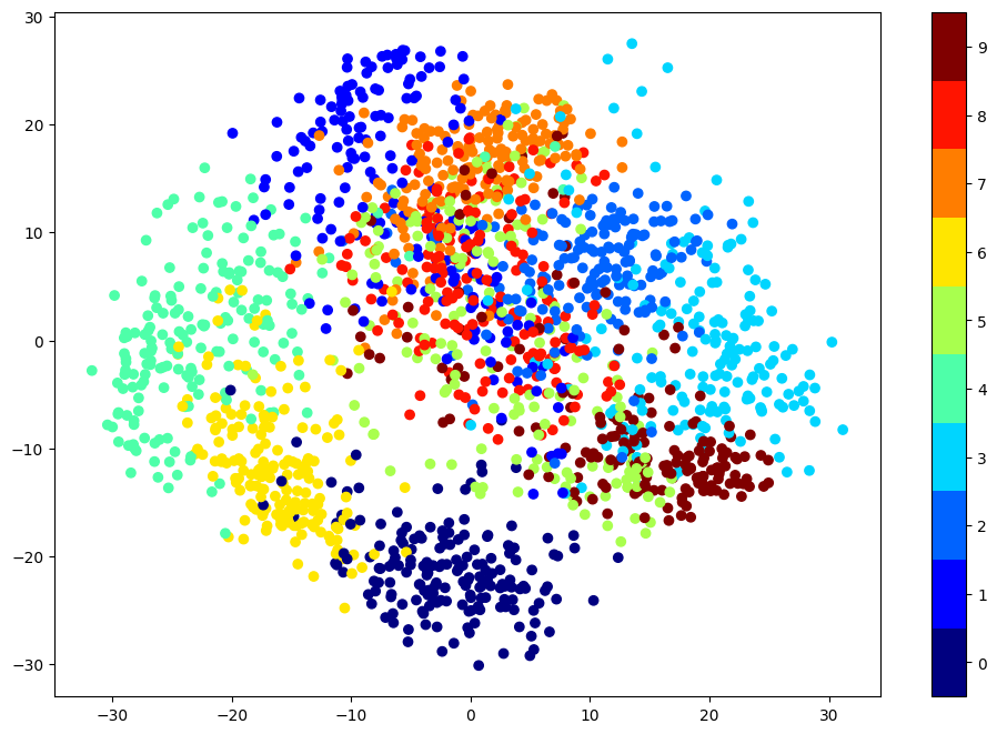
Project the normalized data matrix onto the first two weight vectors.

X2d = X @ QT[0:2,:].T

plt.figure(figsize=(12,8))
plt.scatter(X2d[:,0],X2d[:,1],c=digits['target'],cmap=plt.cm.get_cmap('jet', 10))
plt.colorbar(ticks=range(0,10)); plt.clim([-0.5,9.5]);
plt.show()