Polynomial Interpolation

import numpy as np
import scipy.linalg as la
import matplotlib.pyplot as plt

Given \(d+1\) data points \((t_0,y_0), \dots , (t_d,y_d)\) there exists a unique polynomial of degree \(d\)

\[ p(t) = c_0 + c_1 t + \cdots + c_d t^d \]

such that \(p(t_k) = y_k\) for each \(k=0,\dots,d\). The coefficients \(c_k\) are unknown and each data point gives us an equation

\[\begin{split} \begin{align*} c_0 + c_1t_1 + \cdots + c_d t_1^d &= y_1 \\ c_0 + c_1t_2 + \cdots + c_d t_2^d &= y_2 \\ & \vdots \\ c_0 + c_1t_d + \cdots + c_d t_d^d &= y_d \end{align*} \end{split}\]

This yields a system of equations \(A \boldsymbol{c} = \boldsymbol{y}\)

\[\begin{split} \begin{bmatrix} 1 & t_1 & \cdots & t_1^d \\ 1 & t_2 & \cdots & t_2^d \\ \vdots & \vdots & \ddots & \vdots \\ 1 & t_d & \cdots & t_d^d \end{bmatrix} \begin{bmatrix} c_0 \\ c_1 \\ \vdots \\ c_d \end{bmatrix} = \begin{bmatrix} y_0 \\ y_1 \\ \vdots \\ y_d \end{bmatrix} \end{split}\]

The matrix \(A\) is called a Vandermonde matrix.

Example 1

Start with data points for which we know the solution. Consider \((-1,1),(0,0),(1,1)\). The parabola \(p(t) = t^2\) is the unique polynomial which interpolates these points. Let’s create the system using numpy.vander and solve with scipy.linalg.solve.

t = np.array([-1,0,1])
y = np.array([1,0,1])
A = np.vander(t,increasing=True)

print(A)

[[ 1 -1  1]
 [ 1  0  0]
 [ 1  1  1]]

c = la.solve(A,y)

print(c)

[0. 0. 1.]

The solution corresponds to the coefficients \(c_0=0\), \(c_1=0\) and \(c_2=1\). That is \(p(t) = t^2\).

Example 2

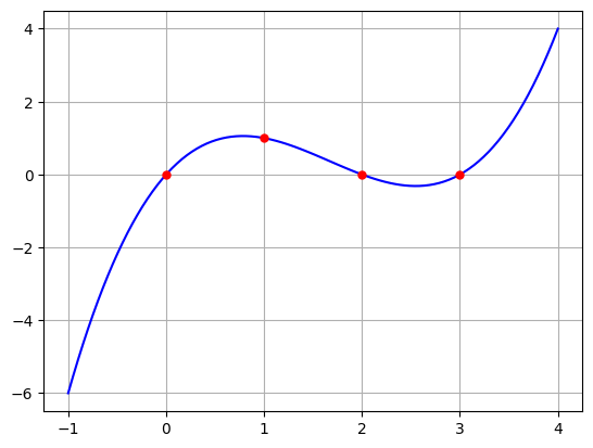
Let’s try a cubic polyniomial which interpolates \((0,0),(1,1),(2,0),(3,0)\).

t = np.array([0,1,2,3])
y = np.array([0,1,0,0])
A = np.vander(t,increasing=True)
c = la.solve(A,y)
print(c)

[ 0.   3.  -2.5  0.5]

T = np.linspace(-1,4,100)
Y = c[0] + c[1]*T + c[2]*T**2 + c[3]*T**3
plt.plot(T,Y,'b-',t,y,'r.',markersize=10)
plt.grid(True)
plt.show()

Example 3

What happens to the condition number as \(N\) increases when \(t_0,t_1,\dots,t_N\) are \(N+1\) equally spaced points from 0 to 1? That is, \(t_k = k/N\), \(k=0,\dots,N\).

C = []
Nmax = 11
for N in range(2,Nmax):
    t = np.linspace(0,1,N+1)
    A = np.vander(t)
    c = np.linalg.cond(A)
    C.append(c)
plt.figure(figsize=(8,5))
plt.plot(range(2,Nmax),C,'b.-',markersize=10)
plt.title('Condition Number of Vandermonde matrix of size N+1')
plt.grid(True)
plt.xlabel('N')
plt.show()

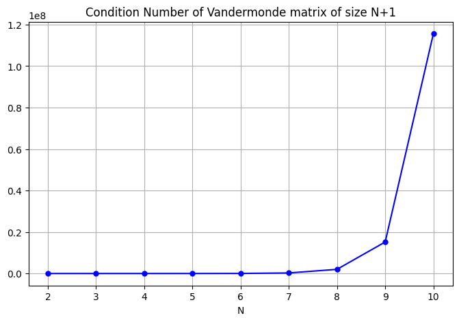
C[-1]

115575244.6289977

The condition number for \(N=10\) is around \(10^8\). Yikes!

Example 4

Let’s interpolate the points \(\sin(\pi t_k)\) for \(t_k = k/N\) for \(N=15\).

N = 15
t = np.linspace(0,1,N+1)
y = np.sin(np.pi*t)
A = np.vander(t,increasing=True)
c = la.solve(A,y)
T = np.linspace(0,1,100)
Y = sum([c[k]*T**k for k in range(0,len(c))])
plt.plot(T,Y,'b-',t,y,'r.',markersize=10)
plt.grid(True)
plt.show()

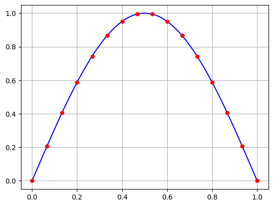
The interpolating polynomial is very nice! But what happens if we introduce some random noise in the data.

N = 15
t = np.linspace(0,1,N+1)
noise = 0.005*np.random.randn(t.size)
y = np.sin(np.pi*t) + noise
A = np.vander(t,increasing=True)
c = la.solve(A,y)
T = np.linspace(0,1,200)
Y = sum([c[k]*T**k for k in range(0,len(c))])
plt.plot(T,Y,'b-',t,y,'r.',markersize=10)
plt.grid(True)
plt.show()

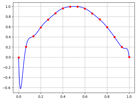
Yikes! The interpolating polynomial is very sensitive to small changes in the \(y\) values! That’s because the condition number is large!