Frequency, Amplitude and Phase#

The DFT of a signal computes the amplitude and phase of each frequency in the signal.

The DFT is used to study sound, images and any kind of information that can be represented by a vector \(\boldsymbol{x} \in \mathbf{C}^N\). Therefore, in the context of the DFT, we use the term signal to refer to a vector \(\boldsymbol{x} \in \mathbf{C}^N\) and we use the notation \(\boldsymbol{x}[n] = x_n\) to refer to the entries

\[\begin{split} \boldsymbol{x} = \begin{bmatrix} \ x_0 \\ x_1 \\ x_2 \\ \vdots \\ x_{N-1} \ \end{bmatrix} \hspace{10mm} \boldsymbol{x}[n] = x_n \end{split}\]

Sinusoids#

Let \(N\) be a positive integer and let

\[\begin{split} \boldsymbol{n} = \begin{bmatrix} 0 \\ 1 \\ 2 \\ \vdots \\ N-1 \end{bmatrix} \hspace{10mm} \boldsymbol{t} = (1/N) \boldsymbol{n} = \begin{bmatrix} 0 \\ 1/N \\ 2/N \\ \vdots \\ (N-1)/N \end{bmatrix} \end{split}\]

A sinusoid is a signal of the form

\[ \boldsymbol{x} = A \cos(2\pi k \boldsymbol{t} + \phi) \]

where \(k\) is the frequency (in periods per \(N\) samples), \(A\) is the amplitude and \(\phi\) is the phase. Here we use vector notation

\[\begin{split} A \cos(2\pi k \boldsymbol{t} + \phi) = \begin{bmatrix} A \cos(\phi) \\ A \cos(2\pi k (1/N) + \phi) \\ A \cos(2\pi k (2/N) + \phi) \\ \vdots \\ A \cos(2\pi k (N-1)/N + \phi) \end{bmatrix} \end{split}\]

Let \(N = 8\) and so

\[\begin{split} \boldsymbol{n} = \begin{bmatrix} 0 \\ 1 \\ 2 \\ 3 \\ 4 \\ 5 \\ 6 \\ 7 \end{bmatrix} \hspace{10mm} \boldsymbol{t} = \begin{bmatrix} 0 \\ 1/8 \\ 1/4 \\ 3/8 \\ 1/2 \\ 5/8 \\ 3/4 \\ 7/8 \end{bmatrix} \end{split}\]

Consider the signal

\[\begin{split} \boldsymbol{x} = \cos(2 \pi \boldsymbol{t} ) = \begin{bmatrix} 1 \\ 1/\sqrt{2} \\ 0 \\ -1/\sqrt{2} \\ -1 \\ -1/\sqrt{2} \\ 0 \\ 1/\sqrt{2} \end{bmatrix} \end{split}\]

and sketch the signal as a stemplot

../_images/stem01.png

Now consider the signal

\[\begin{split} \boldsymbol{x} = \cos(4 \pi \boldsymbol{t} ) = \left[ \begin{array}{r} 1 \\ 0 \\ -1 \\ 0 \\ 1 \\ 0 \\ -1 \\ 0 \end{array} \right] \end{split}\]

and sketch the signal as a stemplot

../_images/stem02.png

DFT of Sinusoids#

The Fourier basis vectors satisfy the following properties:

\[\begin{split} \begin{align*} \boldsymbol{f}_k & = \cos(2 \pi k \boldsymbol{t}) + i \sin(2 \pi k \boldsymbol{t}) \\ \frac{1}{2} \left( \boldsymbol{f}_k + \overline{\boldsymbol{f}}_k \right) &= \cos(2 \pi k \boldsymbol{t}) \\ \frac{1}{2i} \left( \boldsymbol{f}_k - \overline{\boldsymbol{f}}_k \right) &= \sin(2 \pi k \boldsymbol{t}) \end{align*} \end{split}\]

Proof. We showed in a previous proposition that

\[ \omega_N^k = \cos\left( \frac{2 \pi k}{N} \right) + i \sin \left( \frac{2 \pi k}{N} \right) \]

therefore

\[\begin{split} \boldsymbol{f}_k = \renewcommand{\arraystretch}{1.5} \begin{bmatrix} 1 \\ \omega^k_N \\ \omega^{2k}_N \\ \vdots \\ \omega^{(N-1)k}_N \end{bmatrix} = \begin{bmatrix} 1 \\ \cos(2\pi k (1/N)) + i \sin(2\pi k (1/N)) \\ \cos(2\pi k (2/N)) + i \sin(2\pi k (2/N)) \\ \vdots \\ \cos(2\pi k (N-1)/N) + i \sin(2\pi k (N-1)/N) \end{bmatrix} = \cos(2 \pi k \boldsymbol{t}) + i \sin(2 \pi k \boldsymbol{t}) \end{split}\]

Further,

\[\begin{split} \begin{align*} \omega_N^{nk} + \omega_N^{-nk} &= \cos\left( \frac{2 \pi n k}{N} \right) + i \sin \left( \frac{2 \pi n k}{N} \right) + \cos\left( \frac{2 \pi n k}{N} \right) - i \sin \left( \frac{2 \pi n k}{N} \right) \\ &= 2\cos\left( \frac{2 \pi n k}{N} \right) \end{align*} \end{split}\]

Therefore

\[\begin{split} \boldsymbol{f}_k + \overline{\boldsymbol{f}}_k = \begin{bmatrix} 1 \\ \omega^k_N \\ \omega^{2k}_N \\ \vdots \\ \omega^{(N-1)k}_N \end{bmatrix} + \begin{bmatrix} 1 \\ \omega^{-k}_N \\ \omega^{-2k}_N \\ \vdots \\ \omega^{-(N-1)k}_N \end{bmatrix} = \begin{bmatrix} 2 \\ 2\cos( 2 \pi k/N ) \\ 2\cos( 2 \pi n (2k)/N ) \\ \vdots \\ 2\cos( 2 \pi (N-1) k/N ) \end{bmatrix} = 2 \cos(2 \pi k \boldsymbol{t}) \renewcommand{\arraystretch}{1} \end{split}\]

The last equality is proved similarly.

Let \(\boldsymbol{x} = A \cos(2 \pi k \boldsymbol{t} + \phi)\). Then

\[ \mathrm{DFT}(\boldsymbol{x}) = \frac{AN}{2} e^{i \phi} \, \boldsymbol{e}_k + \frac{AN}{2} e^{-i \phi} \, \boldsymbol{e}_{N-k} \]

Proof. We proved in a previous proposition

\[ \cos(2 \pi k \boldsymbol{t} ) = \frac{1}{2} \left( \boldsymbol{f}_k + \overline{\boldsymbol{f}}_k \right) = \frac{1}{2} \left( \boldsymbol{f}_k + \boldsymbol{f}_{N-k} \right) \]

and we also showed that

\[ \mathrm{DFT}( \boldsymbol{f}_k ) = N \boldsymbol{e}_k \]

Compute

\[ \mathrm{DFT}(\cos(2 \pi k \boldsymbol{t} )) = \frac{1}{2} \mathrm{DFT}(\left( \boldsymbol{f}_k + \boldsymbol{f}_{N-k} \right)) = \frac{1}{2} \left( N\boldsymbol{e}_k + N \boldsymbol{e}_{N-k} \right) \]

Similarly, compute

\[ \mathrm{DFT}(\sin(2 \pi k \boldsymbol{t} )) = \frac{1}{2i} \mathrm{DFT}(\left( \boldsymbol{f}_k - \boldsymbol{f}_{N-k} \right)) = \frac{1}{2i} \left( N\boldsymbol{e}_k - N \boldsymbol{e}_{N-k} \right) \]

Use the trigonometric identity

\[ \cos(\alpha + \beta) = \cos \alpha \cos \beta - \sin \alpha \sin \beta \]

to find

\[\begin{split} \begin{align*} \mathrm{DFT}(\boldsymbol{x}) &= \mathrm{DFT}(A \cos(2 \pi k \boldsymbol{t} + \phi)) \\ &= A \cos(\phi) \, \mathrm{DFT}(\cos(2 \pi k \boldsymbol{t})) - A \sin(\phi) \, \mathrm{DFT}(\sin(2 \pi k \boldsymbol{t})) \\ &= \frac{A \cos(\phi)}{2} \left( N\boldsymbol{e}_k + N \boldsymbol{e}_{N-k} \right) - \frac{A \sin(\phi)}{2i} \left( N\boldsymbol{e}_k - N \boldsymbol{e}_{N-k} \right) \\ &= \frac{AN ( \cos(\phi) + i \sin(\phi) )}{2} \, \boldsymbol{e}_k + \frac{AN (\cos(\phi) - i\sin(\phi))}{2} \, \boldsymbol{e}_{N-k} \\ &= \frac{AN}{2} e^{i \phi} \, \boldsymbol{e}_k + \frac{AN}{2} e^{-i \phi} \, \boldsymbol{e}_{N-k} \end{align*} \end{split}\]

Stemplots#

The magnitude stemplot of a complex vector \(\boldsymbol{y} \in \mathbb{C}^N\) is the plot of the magnitude \(| \boldsymbol{y}[n] |\) versus the index \(n\). The angle stemplot of \(\boldsymbol{y}\) is the plot of the argument \(\angle \boldsymbol{y}[n]\) versus the index \(n\).

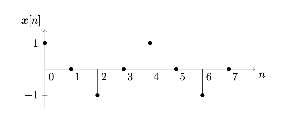
Let \(N=8\) and compute the DFT of the sinusoid \(\boldsymbol{x} = \sin(2 \pi \boldsymbol{t})\). Since \(\boldsymbol{x} = \cos(2 \pi \boldsymbol{t} - \pi/2)\) we have \(A=1\), \(k=1\) and \(\phi = -\pi/2\), and so

\[\begin{split} \boldsymbol{y} = \mathrm{DFT}(\boldsymbol{x}) = -4i \boldsymbol{e}_1 + 4i \boldsymbol{e}_7 = \begin{bmatrix} 0 \\ -4i \\ 0 \\ 0 \\ 0 \\ 0 \\ 0 \\ 4i \end{bmatrix} \end{split}\]

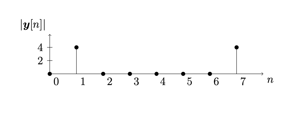
The magnitude stemplot of \(\boldsymbol{y} = \mathrm{DFT}(\boldsymbol{x})\) is given by

../_images/stem03.png

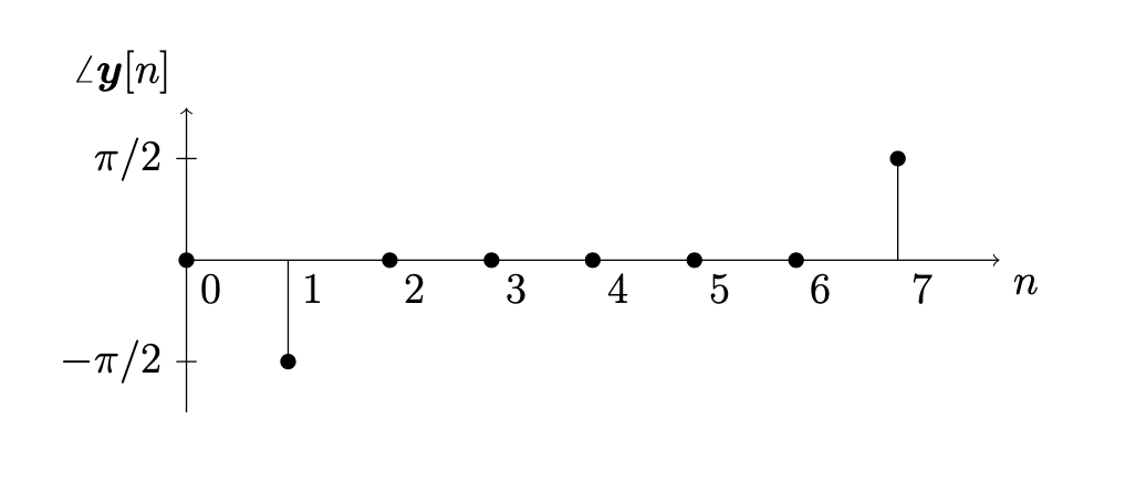
The angle stemplot of \(\boldsymbol{y} = \mathrm{DFT}(\boldsymbol{x})\) is given by
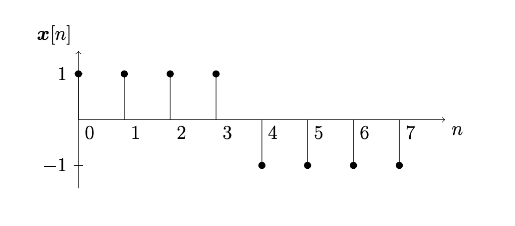
../_images/stem04.png

Let \(N=8\) and let

\[\begin{split} \boldsymbol{x} = \left[ \begin{array}{r} 1 \\ 1 \\ 1 \\ 1 \\ -1 \\ -1 \\ -1 \\ -1 \end{array} \right] \end{split}\]

Sketch the signal

../_images/stem05.png

What frequencies occur in this signal? Compute the DFT

\[\begin{split} \boldsymbol{y} = \mathrm{DFT}(\boldsymbol{x}) = \begin{bmatrix} 0 \\ 2 - 2(\sqrt{2} + 1)i \\ 0 \\ 2 - 2(\sqrt{2} - 1)i \\ 0 \\ 2 + 2(\sqrt{2} - 1)i \\ 0 \\ 2 + 2(\sqrt{2} + 1)i \end{bmatrix} \end{split}\]

The magnitude stemplot of \(\boldsymbol{y}\) is given by

../_images/stem06.png

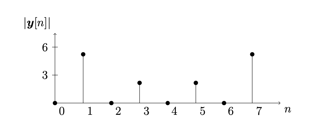
The angle stemplot of \(\boldsymbol{y}\) is given by

../_images/stem07.png

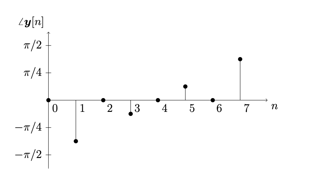
Therefore we may rewrite the signal \(\boldsymbol{x}\) as a sum of sinusoids

\[ \boldsymbol{x} = A_1 \cos(2 \pi \boldsymbol{t} + \phi_1) + A_3 \cos(6 \pi \boldsymbol{t} + \phi_3) \]

where

\[ A_1 = \frac{\sqrt{4 + 2\sqrt{2}}}{2} \hspace{5mm} \phi_1 = -\frac{3 \pi}{8} \hspace{5mm} A_3 = \frac{\sqrt{4 - 2\sqrt{2}}}{2} \hspace{5mm} \phi_3 = -\frac{\pi}{8} \]

Exercises#

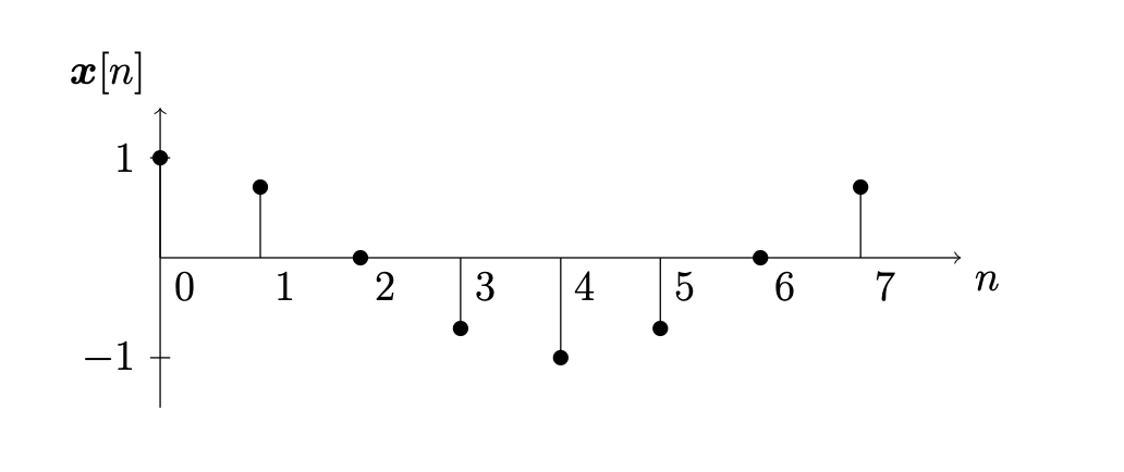
Exercise 1. Find a formula for \(\boldsymbol{x}\) as a sum of sinusoids given

\[ \mathrm{DFT}(\boldsymbol{x}) = \begin{bmatrix} 1 & 3-3i & 2\sqrt{3}+2i& -4i& 4i &2\sqrt{3}-2i & 3+3i \end{bmatrix}^T \]

Exercise 2. Sketch the signal \(\boldsymbol{x}\) such that the magnitude and phase plots of \(\boldsymbol{y} = \mathrm{DFT}(\boldsymbol{x})\) are

../_images/04_02_08.png

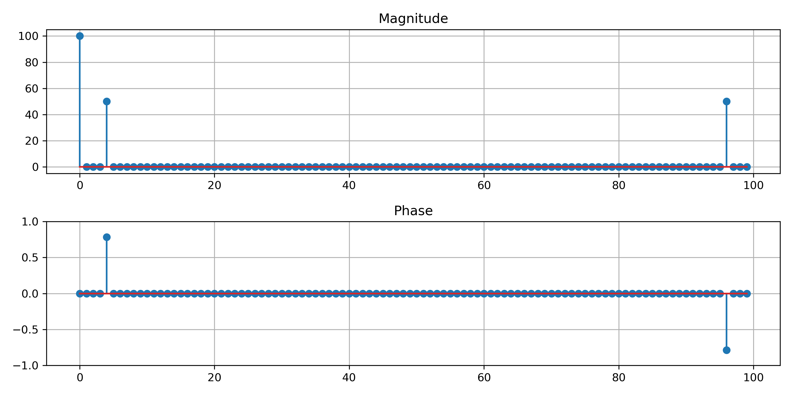
Exercise 3. Run the following Python code for different values \(N\):

N = 100
x = np.random.rand(N)
y = np.fft.fft(x)
plt.stem(np.abs(y),use_line_collection=True)
plt.show()

Describe the magnitude plot and explain why it has the same general shape for each random sample. (Recall np.random.rand samples from the uniform distribution on \([0,1]\).)

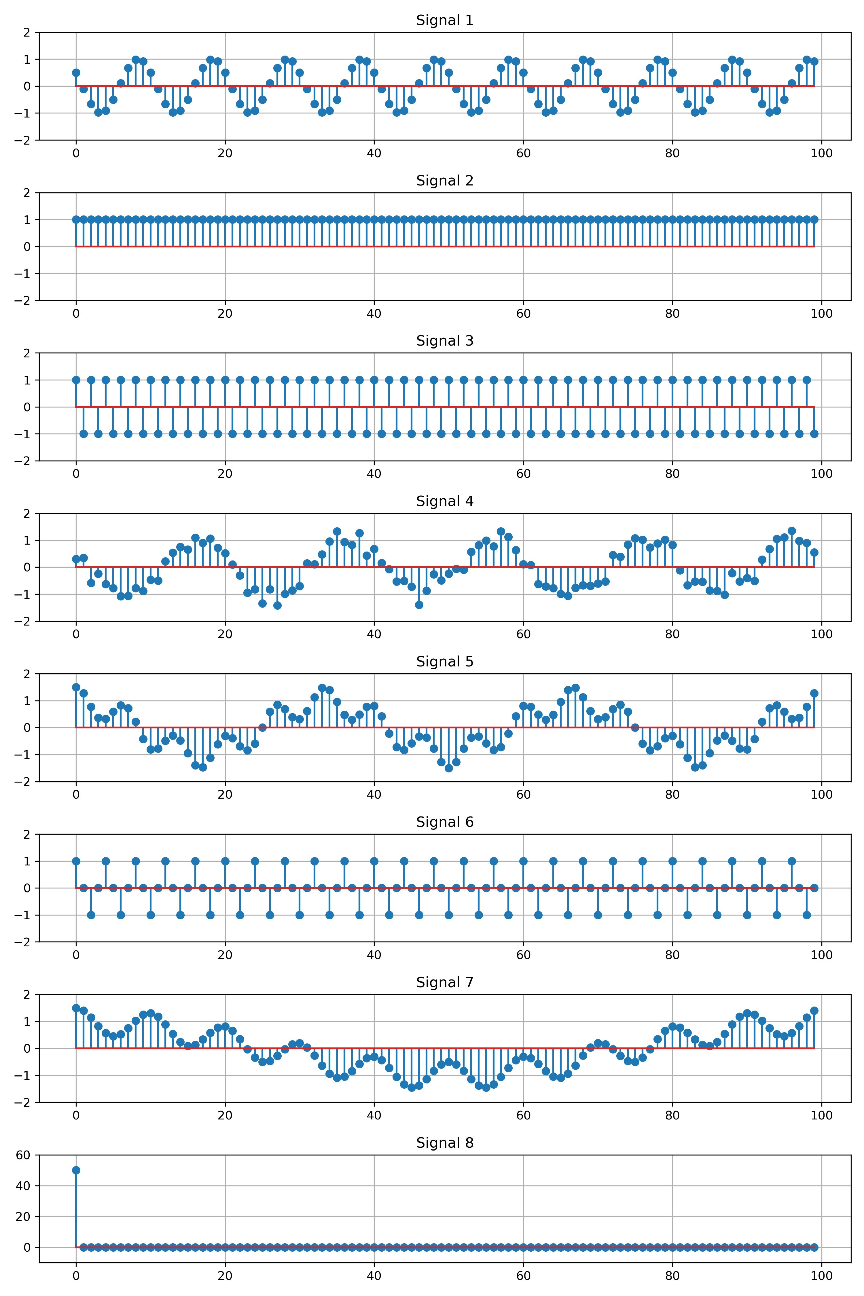
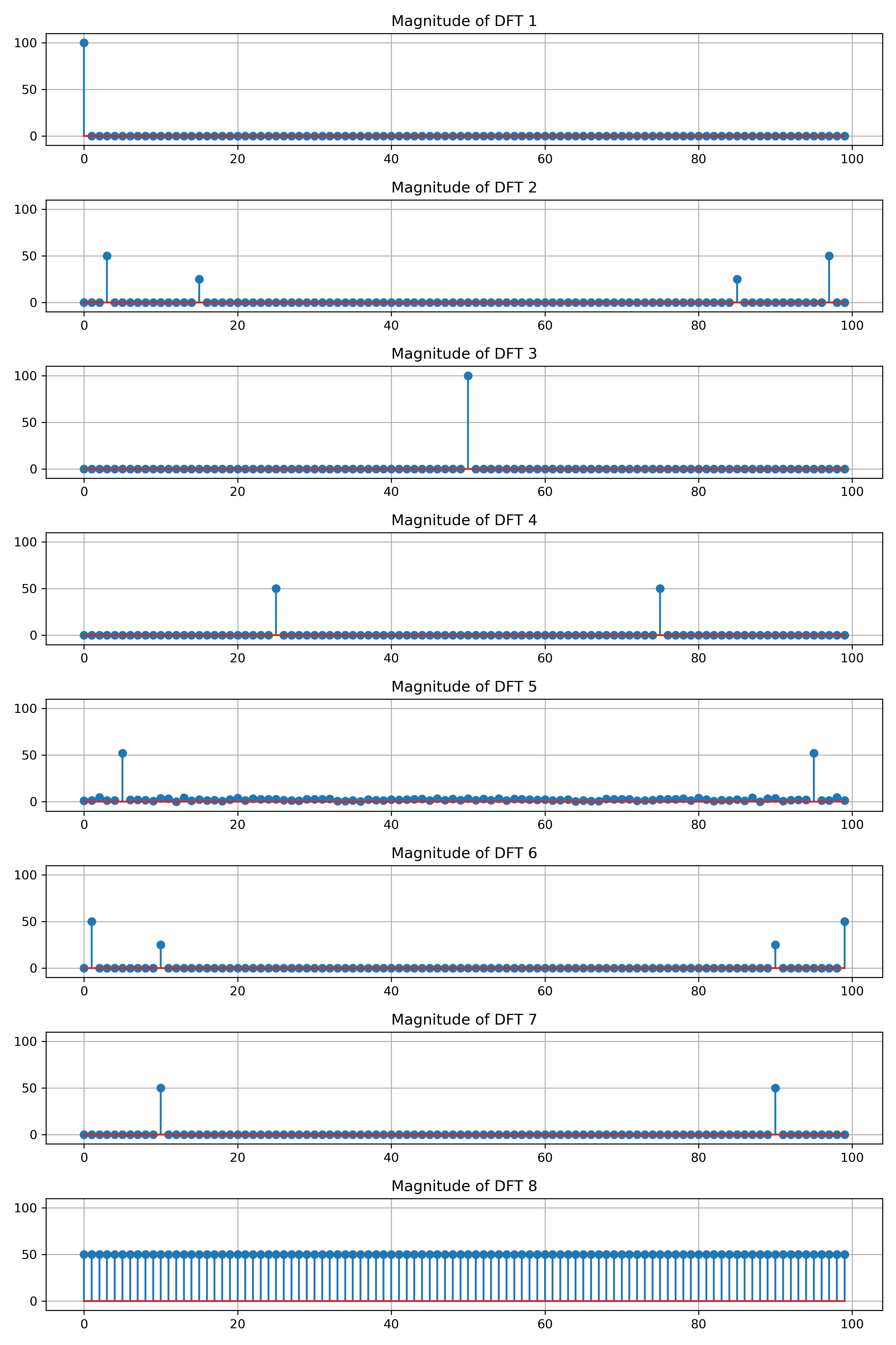
Exercise 4. Match the signal with the magnitude plot of its discrete Fourier transform.

../_images/04_02_09.png ../_images/04_02_10.png